](https://deep-paper.org/en/paper/2502.00816/images/cover.png)
Time series forecasting is one of the oldest mathematical problems humans have tried to solve. From ancient civilizations predicting crop cycles to modern algorithms trading stocks in microseconds, the goal remains the same: use the past to predict the future. However, time series data is intrinsically non-deterministic. No matter how much historical data you have, the future is never a single, fixed point—it is a distribution of possibilities.
In recent years, the success of Large Language Models (LLMs) has prompted researchers to treat time series forecasting as a language problem. If we can predict the next word in a sentence, can’t we predict the next value in a sequence? While this approach has yielded results, it fundamentally forces continuous data (like temperature or stock prices) into discrete “tokens” (like words in a dictionary). This conversion often results in a loss of precision and context.
Enter Sundial, a new family of time series foundation models introduced in a 2025 paper by researchers from Tsinghua University. Sundial proposes a shift away from discrete tokenization and rigid parametric assumptions. instead, it treats time series as native, continuous signals and uses generative modeling—specifically Flow Matching—to predict probable futures.
In this post, we will deconstruct Sundial. We will explore why current foundation models struggle with continuous data, how Sundial’s “TimeFlow” mechanism works, and look at the empirical evidence showing why this might be the new state-of-the-art in forecasting.
The Foundation Model Landscape: Discrete vs. Continuous
To understand why Sundial is significant, we first need to map the current landscape of Time Series Foundation Models (TSFMs). As illustrated below, existing approaches generally fall into two categories, with Sundial carving out a third:
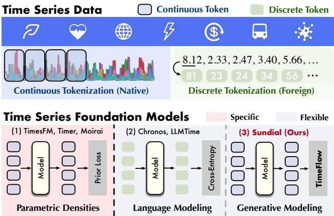
1. Parametric Densities (e.g., TimesFM, Moirai)
These models operate on continuous data but assume the output follows a specific probability distribution (like a Gaussian or Student-t distribution). The model tries to predict the parameters of that distribution (e.g., mean and variance).
- The Problem: Real-world data is messy and heterogeneous. By forcing predictions into a pre-defined mathematical shape, these models often suffer from “mode collapse,” where they default to predicting the average, failing to capture complex, multi-modal possibilities.
2. Language Modeling (e.g., Chronos, LLMTime)
These models treat time series like text. They discretize the data (e.g., turning the value 2.33 into token ID #23).
- The Problem: Time series values have mathematical relationships (2.33 is close to 2.34). When you turn them into discrete tokens, you lose that ordinal relationship. Furthermore, the vocabulary size becomes a bottleneck, and precision is lost during quantization.
3. Generative Modeling (Sundial)
Sundial introduces a “Native” and “Flexible” approach. It keeps the input data continuous (no discretization) and does not assume a fixed output distribution. Instead, it learns to generate the distribution of the next patch of data from scratch using a technique called TimeFlow.
The Sundial Architecture
Sundial is not just a standard Transformer; it is a system designed to handle the specific quirks of time series data. Let’s look at the overall architecture.
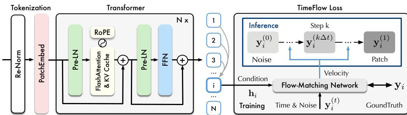
The workflow consists of three distinct stages:
- Tokenization (Patching): Instead of processing data point-by-point, Sundial aggregates time steps into “patches.” This captures local semantic information and reduces the sequence length, making the Transformer more efficient. Crucially, these patches are embedded directly from their continuous values—no quantization is involved.
- Transformer Backbone: The embeddings are fed into a decoder-only Transformer. The authors employ modern optimizations crucial for scaling:
- RMSNorm & Pre-LN: For training stability.
- RoPE (Rotary Positional Embeddings): To better capture relative positions in time.
- FlashAttention & KV Cache: To significantly speed up training and inference memory usage.
- TimeFlow Loss: This is the generative head of the model, which we will detail in the next section.
Handling Arbitrary Lengths
A major challenge in foundation models is handling diverse datasets with different frequencies and lengths. Sundial addresses this via Re-Normalization. Before processing, the input series is normalized to mitigate distribution shifts (non-stationarity). The patch embedding layer then handles arbitrary lengths by padding and masking, ensuring the model can digest anything from short weather patterns to long financial histories.
The embedding process for a patch \(\mathbf{x}_i\) and a binary mask \(\mathbf{m}_i\) (indicating padding) is defined as:

The Core Innovation: TimeFlow Loss
The most technically interesting aspect of Sundial is how it learns to predict the future. The authors propose TimeFlow Loss, based on the concept of Flow Matching.
What is Flow Matching?
Generative models like Diffusion Models work by slowly adding noise to an image (or data) until it is pure noise, and then learning to reverse that process. Flow Matching is a more recent, efficient framework that creates a direct “path” (or flow) between a simple source distribution (like random Gaussian noise) and the complex target distribution (the actual data).
Imagine a field of particles representing random noise. We want to push these particles so they rearrange themselves to look like our target data. The “velocity field” describes the direction and speed each particle needs to move at any given time \(t\) to reach its destination.
The underlying math relies on an Ordinary Differential Equation (ODE):
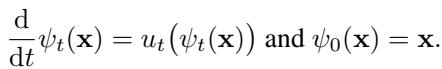
Here, \(\psi_t\) is the position of data at time \(t\), and \(u_t\) is the velocity field.
Conditional Flow Matching for Forecasting
In time series forecasting, we aren’t just generating random data; we are generating the future conditioned on the past. Sundial trains a network to predict the velocity field conditioned on the historical representations learned by the Transformer.
The objective is to minimize the difference between the velocity predicted by the network (\(u_t^{\theta}\)) and the ideal velocity needed to transform noise into the ground truth data (\(\mathbf{y}_i\)).
The general Conditional Flow Matching (CFM) loss is defined as:

By adopting a Gaussian source and an “Optimal Transport” path (the straightest, most efficient path between noise and data), this simplifies mathematically. The training objective for Sundial, conditioned on the history representation \(\mathbf{h}_i\), becomes:
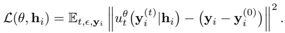
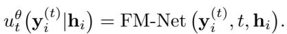
The neural network, called FM-Net (Flow-Matching Network), takes three inputs:
- The noisy data at the current step \(t\).
- The time step \(t\) itself.
- The history representation \(\mathbf{h}_i\) (from the Transformer).
Inference: Generating the Future
Once trained, how does Sundial predict the future? It performs generative forecasting.
- It samples a random noise vector \(\mathbf{x}_0\) from a standard Gaussian distribution.
- It uses the trained FM-Net to calculate the velocity at discrete steps (using an ODE solver).
- It iteratively updates the noise vector, effectively “pushing” it along the flow until it transforms into the predicted future patch.
The update step for a time step \(\Delta t\) looks like this:
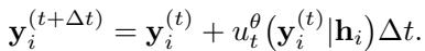
Because the starting point is random noise, running this process multiple times generates multiple different probable predictions. This allows Sundial to quantify uncertainty naturally, without assuming the uncertainty looks like a Bell curve.
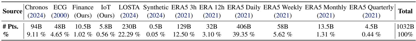
Building TimeBench: A Trillion-Scale Dataset
A foundation model is only as good as its data. To train Sundial, the researchers curated TimeBench, a massive repository containing over 1 trillion time points.
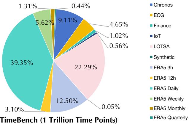
As shown in the chart above, the data is highly diverse:
- Real-world data: Finance, IoT sensor logs, ECG (heart signals), and massive meteorological datasets (ERA5).
- Synthetic data: A small percentage (1.31%) of synthetic kernels is added to enhance pattern diversity and robustness.
The scale here is unprecedented for time series work. Table 4 (below) breaks down the exact counts, showing that Sundial’s training corpus dwarfs those used by previous models like Chronos (94B points) or Lag-Llama.
Experimental Results
The authors evaluated Sundial against the current heavyweights in the field: Time-MoE, Timer, Moirai, Chronos, and TimesFM. They tested on standard benchmarks (TSLib) and probabilistic benchmarks (GIFT-Eval, FEV).
1. Point Forecasting (Zero-Shot)
On the Time-Series-Library (TSLib) benchmark, Sundial was tested in a “zero-shot” setting—meaning it was never trained on these specific datasets.
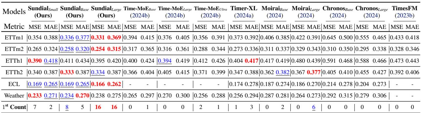
Sundial consistently achieves the lowest Error (MSE and MAE) across datasets like Weather and Electricity (ECL). Notably, it outperforms Time-MoE, a model with significantly more parameters (2.4B vs Sundial’s 444M), highlighting the efficiency of the Generative TimeFlow approach over pure parameter scaling.
2. Probabilistic Forecasting
This is where the generative nature of Sundial shines. By sampling multiple potential futures, Sundial can estimate the probability distribution of the forecast.
Evaluated on the GIFT-Eval benchmark (23 diverse datasets), Sundial achieves top-tier performance in CRPS (Continuous Ranked Probability Score), a metric that measures how well the predicted distribution matches the reality.
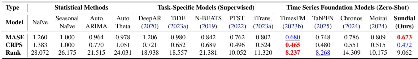
Similarly, on the FEV Leaderboard, Sundial ranks highly among foundation models. It achieves these results while maintaining a critical advantage: speed.
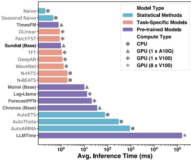
3. Inference Speed
Generative models (like Diffusion) are notoriously slow because they require iterative denoising steps. However, Flow Matching is generally faster than Diffusion because the “path” from noise to data is straighter.
The authors optimized Sundial to be practically usable. As shown in Figure 5, Sundial’s inference speed is orders of magnitude faster than LLM-based approaches (LLMTime) and remains competitive with specialized task-specific models.
4. Generative Capabilities vs. Regression
Why go through the trouble of Flow Matching instead of just using a standard Mean Squared Error (MSE) loss? The answer lies in Mode Collapse.
When a model minimizes MSE, it tends to predict the average of all possible futures to play it safe. This results in “blurry,” over-smooth predictions that miss the natural volatility of time series.
The comparison in Figure 14 is striking. The Left side shows Sundial (TimeFlow), and the Right side shows the same architecture trained with MSE.
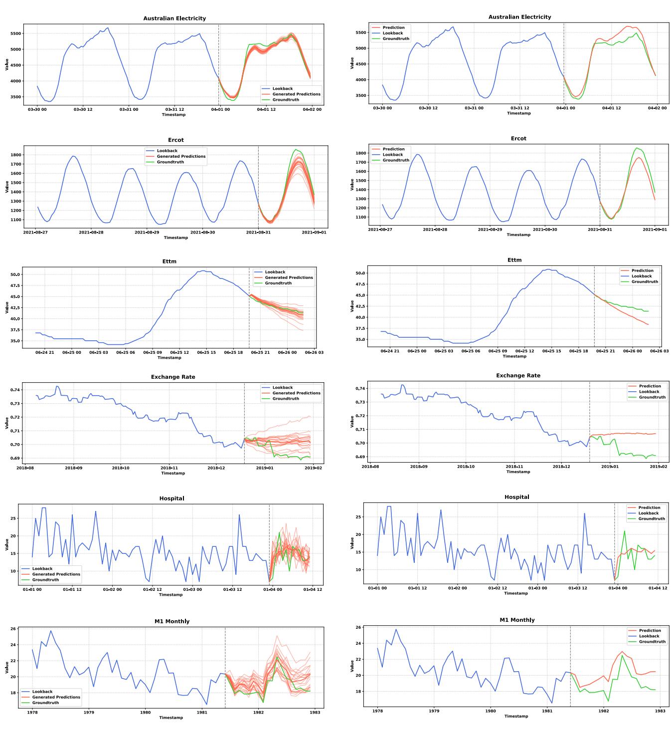
Notice how the MSE predictions (Right) often converge to a smooth, straight line (the mean), completely failing to capture the jagged, oscillating nature of the ground truth. Sundial (Left) generates sharp, varied predictions that resemble the actual dynamics of the data.
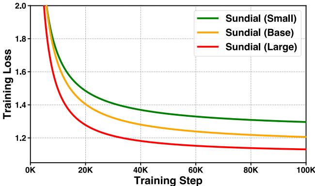
Scalability and Ablations
Does the model follow scaling laws? The authors trained Small (32M), Base (128M), and Large (444M) versions. The training curves indicate that simply increasing model size leads to better convergence and lower loss, suggesting that we haven’t hit the ceiling of what TimeFlow can do yet.
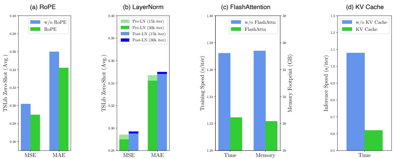
Furthermore, ablation studies confirmed that the architectural choices—specifically RoPE and Pre-LN—were essential for performance. Interestingly, FlashAttention and KV Cache provided massive speedups (reducing inference time by ~43%) without sacrificing any accuracy.
Conclusion
Sundial represents a “third wave” in Time Series Foundation Models. By rejecting the discrete tokenization of Language Models and the rigid parametric assumptions of statistical deep learning, it offers a native, flexible alternative.
The combination of TimeFlow Loss (conditional flow matching) with a massive, diverse dataset (TimeBench) allows Sundial to capture the inherent uncertainty of the future without smoothing over the details. It provides not just a forecast, but a distribution of probable futures, making it a powerful tool for reliable decision-making in unpredictable environments.
As foundation models continue to evolve, Sundial demonstrates that treating continuous data as continuous—rather than forcing it to speak a language it wasn’t designed for—is a path worth following.