In the current landscape of Artificial Intelligence, we rarely train models from scratch. Instead, we stand on the shoulders of giants: we take a massive, pre-trained model (like Llama, Gemma, or ResNet) and “fine-tune” it on a specific dataset to perform a specific task, such as medical diagnosis or mathematical reasoning.

However, there is a ghost in the machine. As models learn new tasks, they have a nasty habit of erasing what they already know. This phenomenon is called Catastrophic Forgetting. You teach a model to solve math problems, and suddenly it forgets how to construct a grammatically correct sentence or loses its general reasoning abilities.

The standard solution has historically been to “replay” old data during the new training phase. But what if you don’t have the old data? In many real-world scenarios, we download a model weights file (e.g., Llama 3) but we do not have access to the petabytes of proprietary internet data used to train it. We are in a data-oblivious setting.

In a recent paper, researchers proposed a counter-intuitive but powerful solution called FLOW (Fine-tuning with Pre-trained Loss-Oriented Weighting). Their insight flips standard machine learning wisdom on its head: instead of focusing on the “hard” examples to learn faster, we should focus on the “easy” examples to remember better.

The Problem: The Fine-Tuning Paradox

Fine-tuning is a delicate balancing act. Ideally, we want to achieve two goals simultaneously:

1. Plasticity: The model must change its parameters to learn the new downstream task.
2. Stability: The model must preserve the representations learned during pre-training to maintain general capabilities.

When we fine-tune using standard methods (like minimizing Cross-Entropy Loss), the optimization algorithm ruthlessly updates parameters to fit the new data. If the new task’s gradients point in a direction orthogonal to the original knowledge, the model drifts away from its pre-trained state.

The Constraints of the “Data-Oblivious” Setting

Most existing techniques to fight catastrophic forgetting assume you know something about the pre-training data.

• Replay Methods: Store a buffer of old images/text and mix them in. (Impossible if you don’t have the data).
• Regularization (e.g., EWC): Penalize changes to important parameters. (Computationally expensive and often requires the Fisher Information Matrix from old data).

The authors of FLOW tackle the hardest version of this problem: You have the pre-trained model (\(\theta^*\)) and the new dataset. Nothing else.

The Core Method: FLOW

The researchers’ proposed solution, FLOW, operates purely in the sample space. It doesn’t require messing with the model architecture or storing gradients. It simply asks: Which samples in the new dataset are “safe” to learn from?

The Intuition: Easy vs. Hard Samples

In standard machine learning, we often prioritize “hard” samples—those with high loss—because they contain the most signal for learning. If the model gets a prediction wrong, we want to correct it.

FLOW takes the opposite approach to mitigate forgetting.

• Easy Samples: These are data points in the fine-tuning set where the pre-trained model already achieves low loss. They are consistent with the model’s existing knowledge.
• Hard Samples: These are data points where the pre-trained model has high loss. Learning these aggressively requires significant changes to the model’s parameters, leading to drift.

The hypothesis is simple: By upweighting the easy samples (where pre-trained loss is low), we introduce a “supervised bias” that keeps the gradients aligned with the pre-trained model.

The Algorithm

The FLOW algorithm is elegant in its simplicity. It consists of three steps:

1. Inference: Pass the new fine-tuning dataset through the frozen pre-trained model.
2. Weighting: Assign a weight \(w_i\) to each sample based on the loss it generated in step 1. Lower loss gets higher weight.
3. Training: Fine-tune the model on the new dataset using these calculated weights.

The Mathematical Foundation

To derive the optimal weighting scheme, the authors frame the problem as an optimization task. We want to find a distribution of weights \(\pi\) that favors samples with low pre-trained loss (\(f_i(\theta^*)\)) while remaining somewhat uniform (we don’t want to train on just one sample).

This is achieved by minimizing the following objective function:

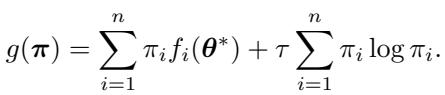
Here, the first term minimizes the weighted loss on the pre-trained model, and the second term is negative entropic regularization, controlled by a temperature parameter \(\tau\). This entropy term ensures the weights don’t collapse to a single point.

Solving this optimization problem using Lagrangian multipliers yields the optimal weight for the \(i\)-th sample:

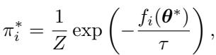
This result is fascinating because it looks like a softmax function, but with a negative sign inside the exponential. It confirms that the weight \(\pi^*_i\) is inversely proportional to the pre-trained loss.

Contrast with Distributionally Robust Optimization (DRO)

It is helpful to contrast FLOW with Distributionally Robust Optimization (DRO). DRO is designed to make models robust by focusing on the worst-case scenarios. Its objective looks like this:

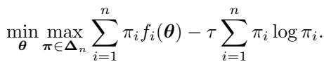
Notice the max over \(\pi\). DRO tries to find the weights that maximize the loss, forcing the model to improve on hard samples. The solution to DRO assigns weights proportional to \(\exp(f_i(\theta)/\tau)\).

FLOW does the exact opposite. It minimizes the drift by clinging to the easy samples. It effectively says, “Let’s learn the new task, but let’s prioritize the data points that don’t force us to fundamentally rewrite our neural pathways.”

Implementing FLOW

In practice, the algorithm is implemented as follows. For a dataset of pairs \((\mathbf{x}_i, \mathbf{y}_i)\):

1. Compute weights: \(w_i = \exp\left(-\frac{f_i(\boldsymbol{\theta}^*)}{\tau}\right)\).
2. Calculate the weighted loss:

3. Minimize this loss to find the fine-tuned parameters \(\widehat{\theta}^*\).

A key heuristic provided by the authors is the choice of the temperature \(\tau\). They set \(\tau\) to the median of the pre-trained losses. This makes the method essentially parameter-free, removing the need for expensive hyperparameter tuning.

Theoretical Analysis: Why it Works

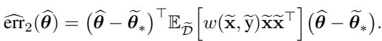
The authors provide a rigorous analysis using linear models to explain the geometric effect of FLOW.

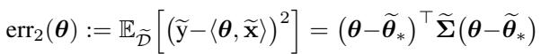
In a linear setting, we can define the total error on the pre-training task (\(\mathrm{err}_1\)) and the fine-tuning task (\(\mathrm{err}_2\)) based on the parameter distance from the optimal solutions.

When we perform standard fine-tuning (Vanilla FT), the model moves rapidly from the pre-trained weights (\(\theta^*\)) toward the fine-tuning optimum (\(\tilde{\theta}^*\)). The analysis shows that this movement is aggressive and cannot be easily impeded.

However, with FLOW, the trajectory changes. The weighting scheme effectively alters the covariance matrix of the data “seen” by the optimizer. The weighted covariance matrix \(\tilde{\Sigma}'\) is derived as:

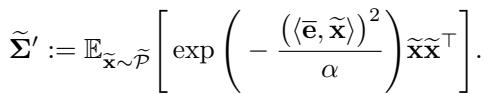
Through a series of derivations involving the eigenvectors of this new matrix, the authors show that FLOW stalls learning in specific directions.

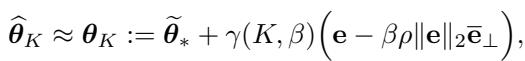
Specifically, FLOW stalls convergence along the direction of the error vector \(\mathbf{e}\). This “stalling” is what prevents the model from overfitting to the fine-tuning task and destroying the pre-trained representations. It essentially acts as a soft brake, allowing the model to adapt without losing its identity.

Experiments and Results

The authors tested FLOW on both computer vision (ResNet) and Large Language Models (Gemma, Llama). The results consistently show that FLOW strikes a superior balance between learning the new task and remembering the old one.

Vision Tasks (ResNet-50)

The team fine-tuned a ResNet-50 model (pre-trained on ImageNet-1K) on several downstream datasets like CIFAR-10, Cars, and Flowers. They measured two things:

1. Target Accuracy: How well does it perform on the new dataset?
2. Pre-training Accuracy: How well does it still perform on ImageNet?

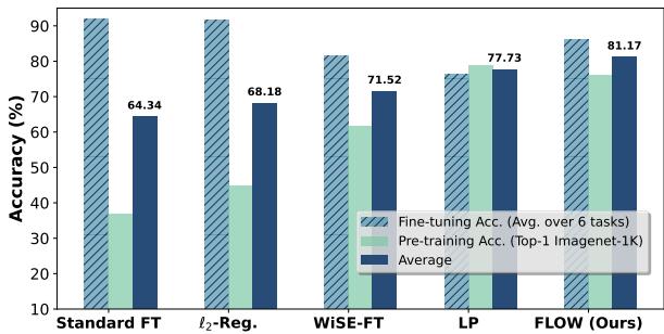
As shown in Figure 1 above, Standard Fine-Tuning (FT) achieves high target accuracy (~87%) but obliterates pre-training performance, dropping from nearly 80% to ~34%.

FLOW (Red bars) maintains a pre-training accuracy of ~77% (almost unchanged!) while still achieving ~85% on the target task. When you look at the Average metric (the grey bars), FLOW is the clear winner, outperforming L2 regularization and WiSE-FT.

To visualize the trade-off, we can look at the scatter plot below. The ideal method would be in the top-right corner (High Fine-tune Accuracy, High ImageNet Accuracy).

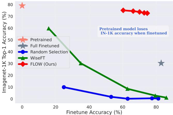
Standard Fine-tuning (the curve moving to the bottom right) gains fine-tuning accuracy but crashes in ImageNet accuracy. FLOW (the red diamonds) stays much higher on the Y-axis, maintaining robustness.

Language Models (LLMs)

The stakes are higher with LLMs. The authors fine-tuned Gemma 2B and Llama 3.2 3B on a math dataset (MetaMathQA) and tested if the models “forgot” general knowledge (tested via benchmarks like MMLU and Commonsense QA).

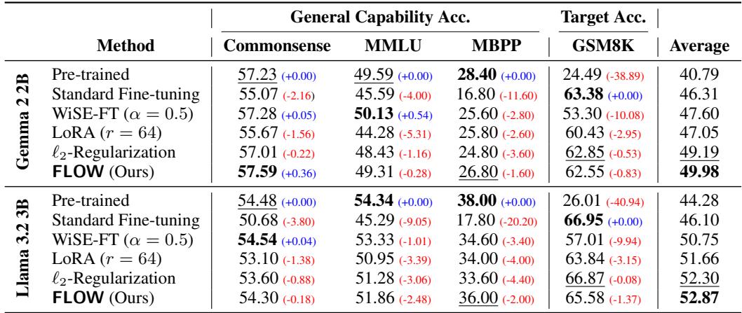
Table 2 highlights the results:

• Standard Fine-Tuning improves Math (GSM8K) scores significantly but causes drops in Commonsense and MMLU scores.
• FLOW achieves Math scores very close to Standard FT (e.g., 62.55 vs 63.38 on Gemma) but preserves significantly more general capability.
• On Llama 3.2, FLOW actually achieves the highest average score across all metrics.

Does it work with other methods?

One of the strongest arguments for FLOW is that it is orthogonal to other methods. You can combine it with parameter-efficient methods like LoRA (Low-Rank Adaptation) or model averaging methods like WiSE-FT.

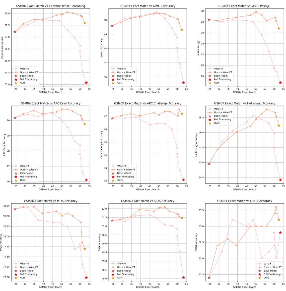
Figure 4 demonstrates that combining FLOW with WiSE-FT (the orange lines) often yields better results than using WiSE-FT alone (pink lines), pushing the performance frontier further toward the ideal top-right corner.

Ablation: Sequence vs. Token Weighting

For LLMs, “samples” can be defined as whole sequences (sentences/paragraphs) or individual tokens. The authors investigated which level of granularity works best.

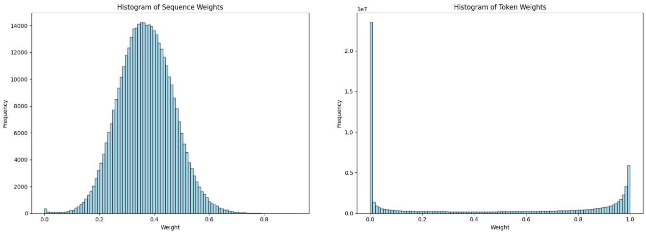
The histograms in Figure 3 reveal a critical insight.

• Left (Sequence Weights): The weights follow a nice Gaussian-like distribution. There is diversity in the weights, allowing the model to prioritize effectively.
• Right (Token Weights): The distribution is extremely skewed. Most tokens get a weight of near-zero or one. This binary behavior over-regularizes the model, preventing it from learning the new task effectively.

Consequently, sequence-wise weighting is the recommended approach for LLMs.

The Cost of FLOW

Is there a catch? Yes. By upweighting easy samples, we are implicitly downweighting hard samples. In the context of the new task, the “hard” samples are often the ones that contain the most novel information or edge cases.

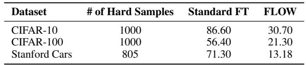
As Table 5 shows, FLOW performs poorly on the specific subset of “hard samples” within the new dataset compared to standard fine-tuning. This is the calculated sacrifice: we accept lower performance on the most difficult outliers of the new task to ensure we don’t catastrophically forget the general capabilities of the pre-trained model.

Conclusion

The “Upweighting Easy Samples” paper provides a refreshing perspective on the problem of catastrophic forgetting. In a field obsessed with hard negatives and difficult examples, FLOW demonstrates that stability comes from the easy path.

By simply calculating the pre-trained loss and re-weighting the new data, we can fine-tune models that learn new tricks without forgetting their old ones. This is a crucial step forward for “Data-Oblivious” AI, allowing us to customize powerful open-source models safely, without needing access to the proprietary data troves of tech giants.

Key Takeaways:

• Concept: Upweight samples that the pre-trained model already “understands” (low loss).
• Method: A simple, parameter-free weighting scheme (\(\tau\) = median loss).
• Result: State-of-the-art mitigation of forgetting in Vision and Language models without accessing old data.
• Implementation: Easy to add to existing training loops and compatible with LoRA and other techniques.