](https://deep-paper.org/en/paper/2502.02990/images/cover.png)
In the era of big data, we are constantly faced with a paradox. On one hand, we need to aggregate information from millions of user devices—smartphones, wearables, and IoT sensors—to understand population trends. On the other hand, this data is often deeply personal. Whether it is salary information, health metrics, or screen-time usage, users (and laws) demand privacy.
How do we calculate simple statistics, like the median salary or the 95th percentile of app usage, without ever collecting the raw data?
This is the challenge of Distributed Private Quantile Estimation. A new research paper, Lightweight Protocols for Distributed Private Quantile Estimation, proposes a breakthrough approach using adaptive algorithms. The researchers demonstrate that by asking questions sequentially—where the next question depends on the previous answer—we can estimate quantiles with significantly fewer users than previously thought possible.
In this post, we will tear down this paper, exploring how Local Differential Privacy (LDP), Noisy Binary Search, and Shuffling can be combined to solve this problem efficiently.
The Problem: Finding the Median Without Seeing the Numbers
Imagine we have \(n\) users. Each user holds a secret number \(x_j\) that belongs to a range \(\{1, \dots, B\}\). For example, if we are looking at salaries, \(B\) might be 1,000,000.
Our goal is to find the median (or any other quantile) of these values. In a non-private world, we would simply collect all numbers, sort them, and pick the middle one. But in our scenario, we cannot see the raw numbers. We must operate under Local Differential Privacy (LDP).
What is Local Differential Privacy?
In the LDP model, the user does not trust the server. Instead of sending their raw data \(x\), the user runs a randomized mechanism \(\mathcal{M}\) on their device and sends the noisy result \(y\).
![Pr[M_i(x)=y] <= e^epsilon * Pr[M_i(x’)=y].](/en/paper/2502.02990/images/004.jpg#center)
The equation above defines \(\varepsilon\)-LDP. Intuitively, it guarantees that the output \(y\) does not reveal too much about the input \(x\). If \(\varepsilon\) (epsilon) is small, the privacy is high, but the data is very noisy. If \(\varepsilon\) is large, the data is accurate, but privacy is lower.
The standard tool for this is Randomized Response. Think of it as flipping a coin before answering a yes/no question. If heads, you tell the truth. If tails, you answer randomly. The server receives a noisy answer but can estimate the true statistics if it has enough users.
The Goal: Empirical Cumulative Distribution Function (CDF)
To find a quantile, we generally look at the Empirical CDF, denoted as \(F_X(i)\). This function tells us what fraction of users have a value less than or equal to \(i\).
![F_X(i) = 1/n * |{j in [n] | x_j <= i}|.](/en/paper/2502.02990/images/001.jpg#center)
If we want the median, we are looking for a value \(m\) where \(F_X(m) \approx 0.5\).
The Innovation: Adaptive vs. Non-Adaptive
Current solutions to this problem are mostly non-adaptive. This means the server decides all the questions it wants to ask before collecting any data. For example, it might ask User 1 about range [0-100], User 2 about [0-100], and User 3 about [100-200].
The researchers highlight a major limitation here: Non-adaptive protocols are inefficient. They require a massive number of users (scaling with \(\text{poly}(\log B)\)) to get an accurate result because they have to “blindly” cover the whole domain.
The researchers propose a Sequentially Adaptive approach.
As shown in the equation above, in an adaptive protocol, the query sent to user \(i\) depends on the answers received from users \(1, \dots, i-1\). This allows the algorithm to “zoom in” on the median, much like a game of High-Low or Binary Search.
Core Method: Noisy Binary Search
The heart of the paper is mapping the problem of private median estimation to Noisy Binary Search.
In a standard Binary Search (like finding a word in a dictionary), you look at the middle page. If your word is alphabetically later, you discard the first half and look at the middle of the second half. You repeat this \(\log B\) times.
In the private setting, we can’t check the “middle page” perfectly. We can ask a user: “Is your value \(\le m\)?” The user will apply LDP (add noise) and say “Yes” or “No”. Because of the noise, we might get the wrong direction.
This transforms the problem into finding a “good coin” in a set of sorted coins with unknown heads-probabilities. We are looking for the threshold \(m\) where the probability of a “Yes” response crosses 0.5.
The Challenge: Sampling Without Replacement
There is a subtle but critical technical hurdle. In standard Noisy Binary Search theory, we assume we can flip the same coin multiple times to get a better estimate. In the LDP user setting, we can only query each user once.
We iterate through the users \(1\) to \(n\). As we consume users, the pool of remaining users gets smaller. This means the true median of the remaining users shifts slightly after every step. The statistical distribution is non-stationary.
The authors solve this by proving that if we process users in a random order, the distribution doesn’t change too much. They model the changing probabilities using a Martingale.
![Pr[max |X_i| >= t] <= 2 exp(-t^2 n / 2).](/en/paper/2502.02990/images/011.jpg#center)
By applying Azuma’s Inequality (shown above), they prove that the deviation of the empirical probabilities (the “coin flips”) remains bounded. Specifically, they show that the probability of the count deviating significantly drops exponentially.
![Pr[max |p_j^t - p_j^0| >= alpha] <= 2 exp(-C log B / 2).](/en/paper/2502.02990/images/018.jpg#center)
This bound allows them to treat the shifting distribution as an Adversarial Noisy Binary Search. Even though the “coin probabilities” (the fraction of people \(\le m\)) wiggle around as we remove users, they stay within a bounded range (\(\alpha\)).
The Algorithm: BayeSS
The researchers utilize an algorithm called BayeSS (Bayesian Screening Search). Instead of a simple binary search, BayeSS maintains a probability distribution (a belief) over where the median might be.
- It selects a query point that splits this belief mass effectively.
- It queries a user: “Is your value \(\le\) query point?”
- It updates the belief based on the noisy response.
By combining the Martingale analysis with BayeSS, the authors derive their first main result. They can find an \(\alpha\)-approximate median using only:
\[O\left(\frac{\log B}{\varepsilon^2 \alpha^2}\right) \text{ users.}\]This is a significant improvement over non-adaptive methods, which require multiplying factors of \(\log B\).
The result is a median \(\tilde{m}_q\) that satisfies the accuracy condition with high probability:
![Pr[[F_X(m_q), F_X(m_q+1)] intersect (q - alpha, q + alpha) != empty] >= 1 - beta.](/en/paper/2502.02990/images/006.jpg#center)
The Shuffle Model: A Middle Ground
Pure LDP is very restrictive (high noise). A popular alternative is the Shuffle Model. Here, users send their noisy messages to a “Shuffler” (a trusted intermediary) that strips away identifiers and randomly permutes the messages before sending them to the analyzer.
Shuffling “hides in the crowd,” amplifying privacy. However, shuffling requires a batch of messages to work. You can’t shuffle a single message. This conflicts with the fully adaptive method described above, which queries one user at a time.
The authors propose a hybrid: Multi-Round Shuffle DP. Instead of querying 1 user at a time, they query a batch of users. They shuffle this batch, analyze the results, and then decide the query for the next batch.
They use Amplification by Shuffling results to show that the privacy guarantee improves significantly.
![Pr[(M_t(x_pi(i))) in S] <= e^epsilon * Pr[…] + delta.](/en/paper/2502.02990/images/008.jpg#center)
This formula shows that the shuffled output satisfies \((\varepsilon, \delta)\)-DP, even if the local mechanism \(\varepsilon_L\) is much weaker (larger).
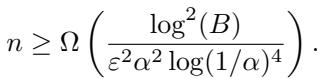
The resulting sample complexity for the Shuffle model is:
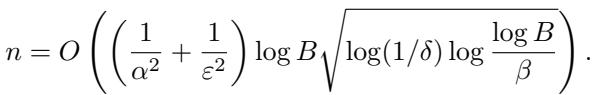
This protocol essentially runs a “Naive” binary search (splitting the domain in half) but uses the privacy amplification of shuffling to require much less noise per user, and therefore fewer users overall.
Experiments: Does it Work?
The authors validated their theoretical bounds with experiments using synthetic data (Pareto and Uniform distributions). They compared their adaptive method (DpBayeSS) against a Naive Noisy Binary Search (DpNaiveNBS) and a state-of-the-art non-adaptive method called the Hierarchical Mechanism.
Success Rate vs. Privacy
In the plot below, we see the success rate (y-axis) as the privacy budget \(\varepsilon\) increases (x-axis). Remember, higher \(\varepsilon\) means less noise.
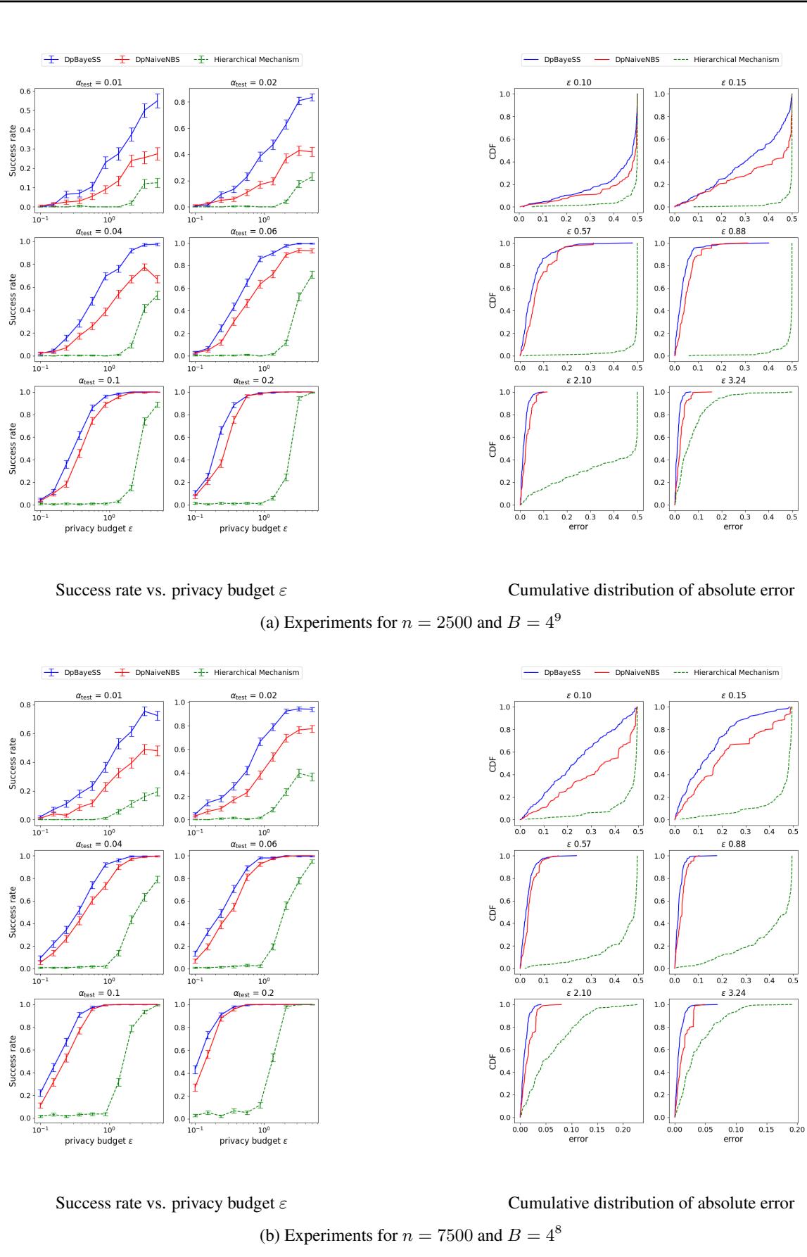
The Blue line (DpBayeSS) consistently achieves a higher success rate than the Red (Naive) and Green (Hierarchical) lines, especially in high-privacy (low \(\varepsilon\)) regimes. The Hierarchical mechanism often fails to return a meaningful median given the number of users, illustrating the “cost” of being non-adaptive.
Stability across Domain Sizes
One of the major theoretical claims is that the adaptive method scales logarithmically with the domain size \(B\).
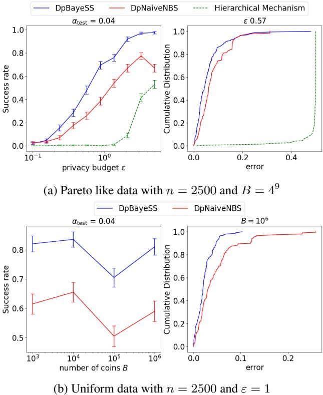
In Figure 1 (above), the left plots show the success rate as the domain size \(B\) increases from \(10^3\) to \(10^6\). The adaptive DpBayeSS (Blue) maintains a high success rate, whereas the Naive approach (Red) degrades more rapidly. This validates that the adaptive “zooming in” capability is crucial when the range of possible values is large.
Lower Bounds: Theoretical Limits
Finally, the paper asks a fundamental question: Is adaptivity actually necessary? Could a clever non-adaptive protocol achieve the same results?
The authors prove a separation result. They demonstrate mathematically that any non-adaptive protocol must use more users (by a factor of \(\log B\)) than the optimal adaptive protocol.
They derive this by connecting the non-adaptive median problem to the problem of learning the entire CDF, which is known to be “harder” in terms of sample complexity.
This lower bound proves that the efficiency gains achieved by their adaptive algorithm are not just an improvement—they are leveraging a fundamental advantage of interaction.
Conclusion
The research presented in Lightweight Protocols for Distributed Private Quantile Estimation offers a significant step forward for federated analytics.
- Optimality: They provide an adaptive LDP algorithm that finds the median with an optimal number of users \(O(\log B)\).
- Robustness: By using martingale arguments, they solve the practical issue of “sampling without replacement,” making the theoretical binary search applicable to real-world user pools.
- Flexibility: They offer a Shuffle DP variant that balances the benefits of batching with the privacy amplification of shuffling.
For students and practitioners in privacy-preserving machine learning, this highlights a key lesson: Interactiveness matters. If your infrastructure allows you to ask questions sequentially rather than all at once, you can achieve the same accuracy with vastly less data—or better accuracy with the same amount of data—while maintaining strict privacy guarantees.