The Transformer architecture has undeniably revolutionized deep learning. From LLMs like GPT-4 to vision models, the “Attention is All You Need” paradigm is ubiquitous. Yet, despite their massive success, we are still playing catch-up in understanding why they work so well. How does a mechanism designed for machine translation become a general-purpose in-context learner?

One of the most compelling theories gaining traction links Transformers to associative memory—specifically, Dense Associative Memory (DAM) or modern Hopfield Networks. The idea is that the attention mechanism isn’t just “attending” to parts of a sequence; it is performing an energy minimization step to retrieve memories.

In this post, we will dive deep into a paper by Smart, Bietti, and Sengupta that refines this connection. They introduce a framework called In-Context Denoising. Their findings are elegant and surprising: they prove mathematically and empirically that a single-layer Transformer can act as a Bayes-optimal denoiser, and that the attention operation corresponds exactly to a single step of gradient descent on a specific energy landscape.

If you are a student of machine learning or physics, this paper bridges the gap between statistical inference, deep learning architectures, and energy-based models.

1. The Setup: What is In-Context Denoising?

To understand what the Transformer is doing, the authors strip the problem down to its basics. Instead of predicting the next word in a Shakespeare sonnet, let’s look at a fundamental signal processing task: Denoising.

In standard In-Context Learning (ICL), a model is given a sequence of examples and asked to predict the output for a new query. The authors generalize this to an unsupervised setting.

The Problem Formulation

Imagine a prompt consisting of a sequence of “clean” tokens \(X_1, \dots, X_L\) drawn from some data distribution. At the end of the sequence, we append a “query” token \(\tilde{X}\) which is a noise-corrupted version of a clean token \(X_{L+1}\).

The goal of the model is simple: look at the context (the clean tokens), look at the noisy query, and predict the original clean token \(X_{L+1}\).

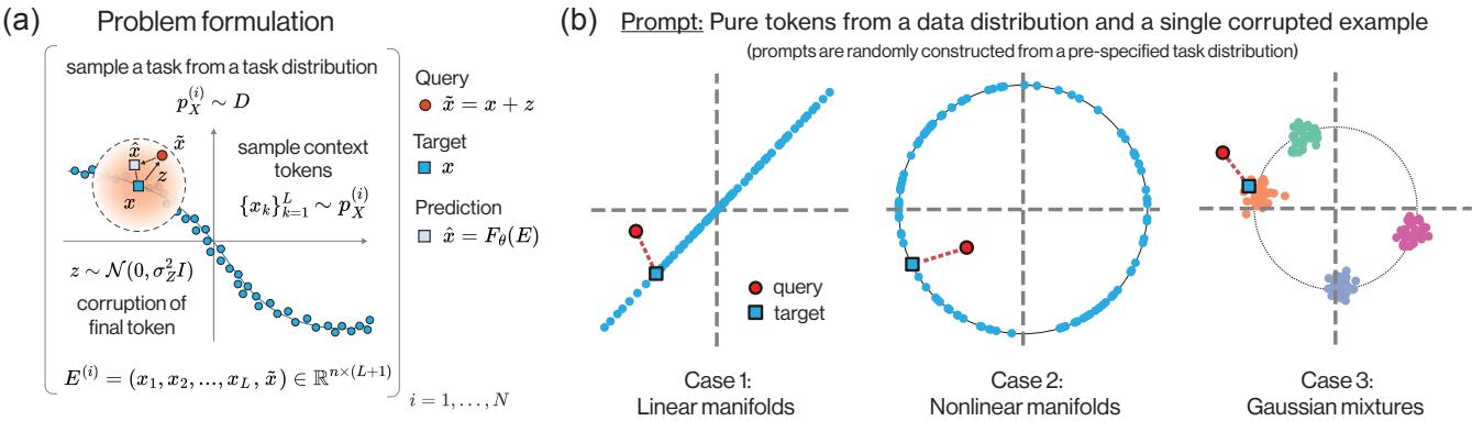
As shown in Figure 1 above, the input \(E^{(i)}\) contains the clean context and the noisy query. The model must output a clean version of the query.

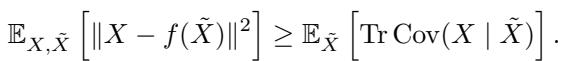
Mathematically, the objective is to minimize the expected loss (usually Mean Squared Error) between the model’s prediction and the ground truth:

Why is this interesting? Because if the noise is random, the model cannot simply “memorize” the answer. It must look at the context to understand the underlying structure (the manifold) of the data distribution, and then project the noisy query onto that structure.

The Three Tasks

The authors test this on three specific types of data distributions, representing common geometric structures in high-dimensional data:

1. Linear Manifolds: Data points lie on a random lower-dimensional subspace (a line or plane).
2. Nonlinear Manifolds: Data points lie on a sphere.
3. Gaussian Mixtures: Data points form distinct clusters.

For each task, the context tokens define the specific geometry (e.g., this specific line, or these specific cluster centers) for that prompt. The model must learn the algorithm to denoise any line or cluster arrangement given in the context.

2. The Gold Standard: Bayes Optimal Denoising

Before training any neural networks, we need a baseline. What is the theoretically “best possible” answer? In statistics, this is the Bayes Optimal predictor. For Mean Squared Error loss, the optimal predictor is the posterior mean—the expected value of the clean data \(X\) given the noisy observation \(\tilde{X}\) and the context.

The authors derive the exact analytical form of the Bayes optimal predictor for the three tasks mentioned above. This is crucial because it gives us a mathematical target to compare against the Transformer’s behavior.

Linear Case: The “Shrunk” Projection

If the data lies on a linear subspace (like a plane in 3D space), and you have a noisy point off that plane, the best guess is to project the point orthogonally onto the plane. However, because there is noise, we must also account for uncertainty. The optimal solution is a shrunk projection: you project the point, but also scale it slightly based on the signal-to-noise ratio.

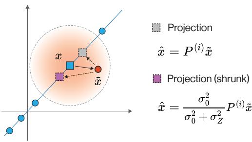
As visualized in Figure 2, the projection \(P^{(i)}\tilde{x}\) (the gray box) puts the point on the line. The Bayes optimal solution (the purple box) scales this by a factor \(\frac{\sigma_0^2}{\sigma_0^2 + \sigma_Z^2}\).

Nonlinear and Clustering Cases

Things get interesting with nonlinear manifolds (spheres) or clusters. The optimal answer isn’t a simple matrix projection anymore. It takes the form of a weighted average over the context points.

For the clustering case (Gaussian mixtures), the optimal predictor looks like this:

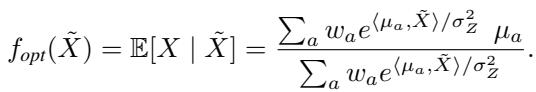
Look closely at that equation. It calculates a weight for each component based on an exponential of the dot product \(\langle \mu_a, \tilde{X} \rangle\), and then computes a weighted sum.

Does this look familiar? It should. It looks suspiciously like the Softmax Attention mechanism in Transformers.

3. The Transformer Solution

Now that we know the mathematical ideal, let’s look at the architecture. The authors examine a one-layer Transformer with a single attention head.

The equation for a standard softmax attention layer, predicting the output \(\hat{X}\), is:

Here:

• \(X_{1:L}\) are the context tokens (acting as Values \(V\) and Keys \(K\)).
• \(\tilde{X}\) is the query (acting as Query \(Q\)).
• \(W_{PV}\) and \(W_{KQ}\) are the learnable weight matrices.

The “Ah-Ha” Moment

Compare the Transformer equation above with the Bayes optimal solution for the clustering/sphere case derived earlier:

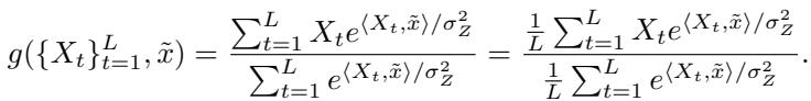
The structure is identical.

• The Bayes solution computes weights using \(e^{\langle X_t, \tilde{x} \rangle / \sigma_Z^2}\).
• The Transformer computes weights using \(\text{softmax}(X_t^T W_{KQ} \tilde{x})\).

If the Transformer sets its weight matrices \(W_{KQ}\) and \(W_{PV}\) to be scaled identity matrices, it exactly recovers the Bayes optimal estimator. specifically, if \(W_{KQ} \approx \frac{1}{\sigma_Z^2} I\) and \(W_{PV} \approx I\).

Empirical Verification: Do they actually learn this?

Theory is nice, but does a randomly initialized Transformer actually learn to become a Bayes optimal denoiser via gradient descent?

The authors trained one-layer transformers on the three tasks. The results are displayed in Figure 3.

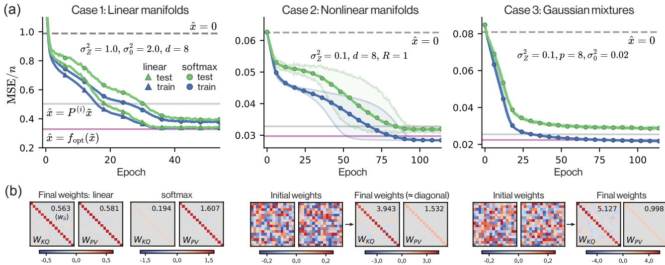
Panel (a) shows the loss curves. The pink line is the theoretical Bayes optimal loss. The circles (softmax attention) converge almost perfectly to this optimal line.

Panel (b) shows the learned weights. This is the smoking gun. The matrices \(W_{KQ}\) and \(W_{PV}\) are not random messes of numbers. They are diagonal matrices. For the linear case, their product converges to the theoretical scaling factor. For the nonlinear cases, they approach the identity structure required by the Bayes optimal formulas.

This confirms that for these denoising tasks, a single self-attention layer naturally evolves into the optimal statistical estimator.

Robustness and Context Length

The authors further explored how “smart” this learned estimator is. Does it get better with more context?

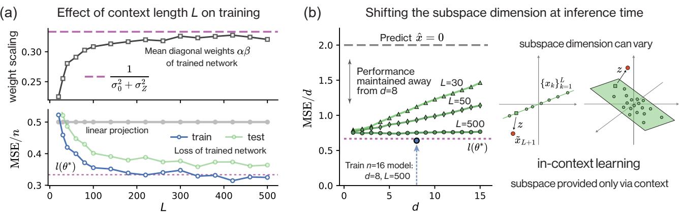
Figure 4(a) shows that as the context length \(L\) increases, the trained network’s weights (squares) and performance (triangles/circles) asymptote toward the theoretical optimum.

Furthermore, Figure 4(b) shows something remarkable about In-Context Learning. A model trained to denoise 8-dimensional subspaces can successfully denoise subspaces of different dimensions at inference time, provided it has enough context tokens to identify the subspace. The model hasn’t just memorized “8D subspaces”; it has learned the algorithm of projection.

4. The Physics Connection: Dense Associative Memory

We have established that the Transformer acts as a Bayesian denoiser. Now, let’s connect this to the paper’s second major contribution: the link to Associative Memory.

Classic Hopfield Networks store memories as fixed points (minima) in an energy landscape. To retrieve a memory, you start with a noisy pattern and iteratively move “downhill” on the energy landscape until you hit a memory.

Modern Hopfield Networks (Dense Associative Memories) use a steeper energy function (often involving exponentials) to drastically increase storage capacity.

The Context-Aware Energy Landscape

The authors define a specific energy function \(\mathcal{E}\) based on the context tokens \(X_{1:L}\) and a state vector \(s\):

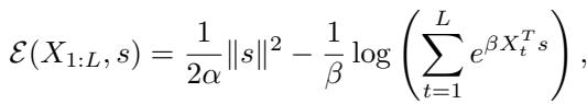
This energy function has two parts:

1. A quadratic term \(\frac{1}{2\alpha}\|s\|^2\) (keeping the state bounded).
2. A Log-Sum-Exp term (the “modern Hopfield” term) that pulls the state toward the context tokens.

Attention = One Gradient Step

If we take the gradient of this energy function with respect to \(s\) and perform a single update step of Gradient Descent (GD), what do we get?

Let’s look at the update rule derived in the paper:

If we initialize the state \(s(0)\) as our noisy query \(\tilde{x}\) and set the step size \(\gamma = \alpha\), the first term \((1 - \frac{\gamma}{\alpha})s(t)\) vanishes. We are left with:

This is exactly the equation for the attention layer we saw earlier!

Why Just One Step?

Standard Hopfield networks usually iterate until convergence (many steps). Why does the Transformer only do one step?

The paper argues that for denoising, you don’t want to converge to a single memory. If you have a noisy input, converging to the nearest memory (a “hard” decision) might be wrong. The Bayes optimal strategy is to find the posterior mean—a weighted blend of likely memories.

The authors visualize this beautifully in Figure 5.

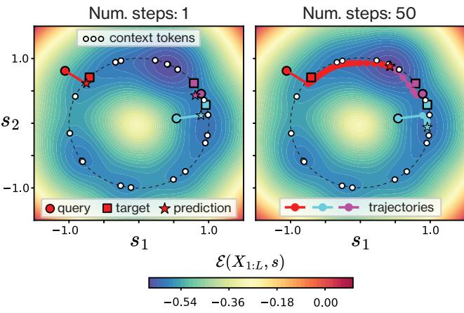
• Left Panel: Shows the result after 1 step (Attention). The star (prediction) moves from the red circle (query) towards the cluster of context tokens, landing right on the target (square). It finds the weighted center.
• Right Panel: Shows what happens if you keep iterating (standard Hopfield retrieval). The points drift deeper into the energy wells, effectively “snapping” to specific context tokens. While good for exact retrieval, this is actually worse for denoising because it ignores the uncertainty represented by the spread of the context.

This provides a powerful intuition: A single attention layer constructs a context-dependent energy landscape and takes one optimal step down the gradient to estimate the posterior mean.

5. Analyzing the Loss Landscape

To further confirm that the Transformer finds this specific solution, the authors analyzed the loss landscape of the training objective. By fixing the weights to be scaled identity matrices (\(\alpha I\) and \(\beta I\)), they plotted the Mean Squared Error (MSE) as a function of \(\alpha\) and \(\beta\).

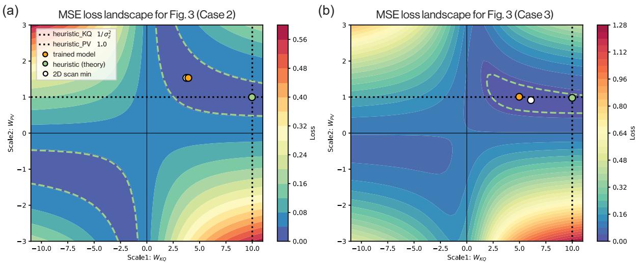
Figure 6 shows these landscapes.

• The Green Dot is the theoretical Bayes optimal setting.
• The Orange Dot is where the trained Transformer ended up.
• The White Dot is the numerical minimum of the landscape.

Notice how they all inhabit the same low-loss “valley.” The broad, hyperbolic shape of the blue valley suggests there is a relationship between \(\alpha\) and \(\beta\) (a multiplicative tradeoff). This explains why the model reliably finds the solution: the “basin of attraction” for the optimal solution is huge.

6. Advanced: Warped Geometries

Finally, the authors asked: what if the world isn’t isotropic? What if the data is stretched or rotated by some transformation matrix \(A\)?

In this case, simple identity matrices for weights won’t work. The optimal weights need to encode the geometry of the transformation:

The weights \(W_{PV}\) and \(W_{KQ}\) should become inverses of the transformation correlation matrices.

Remarkably, the one-layer Transformer learns this too.

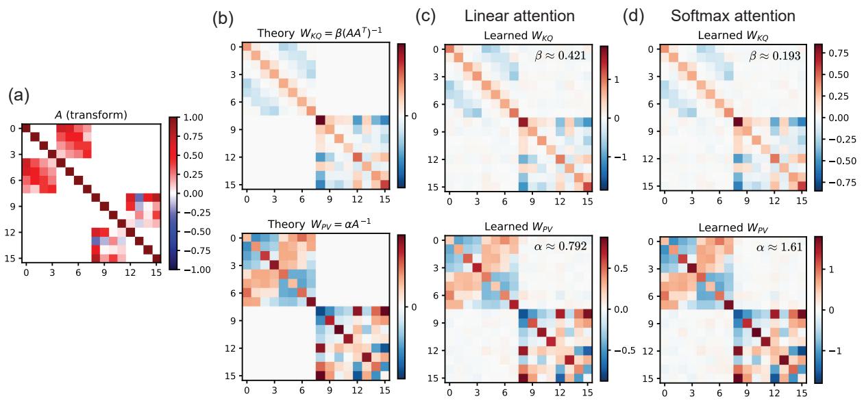
In Figure 8:

• Panel (a) shows the transformation matrix \(A\).
• Panel (b) shows the theoretical optimal weights (structured, not diagonal).
• Panels (c) and (d) show the weights actually learned by the Linear and Softmax attention layers respectively. They recover the complex structure required to undo the transformation \(A\).

This demonstrates that the Transformer isn’t just averaging nearby points; it is learning the metric space in which to perform the averaging.

Conclusion

This paper by Smart et al. provides a rigorous, unifying view of Transformers, Bayesian inference, and Associative Memory.

Here are the key takeaways:

1. Transformers are Denoisers: A fundamental capability of the self-attention mechanism is In-Context Denoising.
2. Optimality: A single layer is expressive enough to implement the Bayes Optimal estimator for linear and spherical manifolds.
3. Mechanism: The learned weights naturally converge to configurations that implement this optimal estimation (scaled identity matrices).
4. Energy Interpretation: The attention operation is mathematically equivalent to a single gradient descent step on a context-defined energy landscape. The query initializes the descent, and the single step moves it to the posterior mean.

This work helps demystify the “black box.” When a Transformer processes a prompt, it isn’t just matching patterns; it is dynamically constructing an energy landscape based on the context and performing an inference step to find the most likely completion. It bridges the gap between the clean, geometric world of vector spaces and the messy, high-dimensional reality of deep learning.