How Mirror Symmetry Can Slice Your Neural Network's Compute in Half

If you have been following the trajectory of deep learning over the last decade, you are likely familiar with “The Bitter Lesson” by Rich Sutton. The core argument is simple: historically, the only technique that consistently matters in the long run is scaling computation. Human ingenuity—hand-crafting features or encoding domain knowledge—eventually gets crushed by massive models trained on massive compute.

But what if we could use human knowledge to improve how we scale computation?

This is the central question behind the research paper “Flopping for FLOPs: Leveraging Equivariance for Computational Efficiency.” The authors challenge the idea that incorporating geometric priors (like symmetry) effectively “taxes” the computational budget. Instead, they propose a method to build neural networks that respect symmetry (specifically mirror symmetry) while cutting the number of floating-point operations (FLOPs) per parameter in half.

In this post, we will dive deep into how this works. We will explore the mathematics of equivariance, how to block-diagonalize linear layers, and how to adapt modern architectures like Vision Transformers (ViT) and ConvNeXts to run faster by simply understanding that a butterfly looks the same when reflected in a mirror.

The Problem with Symmetry and Scale

In computer vision, we know that objects generally retain their identity regardless of orientation. A cat facing left is the same class as a cat facing right.

Standard neural networks, like a vanilla ResNet or ViT, don’t inherently “know” this. They have to learn it by seeing thousands of left-facing cats and thousands of right-facing cats. This is inefficient in terms of parameters (the weights needs to store information for both orientations).

To solve this, researchers developed Equivariant Neural Networks. These networks hard-code symmetry into the architecture. They guarantee that if you transform the input (e.g., rotate or flip it), the internal features transform in a predictable way.

Historically, there has been a catch. While equivariant networks are parameter efficient (they need fewer weights to learn the same task), they are often compute heavy. In many implementations, enforcing symmetry requires weight sharing that results in dense computations. You might save memory on parameters, but you pay for it in FLOPs (Floating Point Operations) and wall-clock time.

The researchers behind “Flopping for FLOPs” asked: Can we design an equivariant network that actually reduces the computational burden?

The Core Solution: Flopping and Block Diagonals

The specific symmetry this paper tackles is horizontal mirroring, which the authors charmingly refer to as “flopping.”

The intuition is to stop thinking about features as generic numbers and start thinking about them as having geometric “types.” When you look at a feature map in a neural network, the authors propose splitting the channels into two distinct groups:

1. Invariant Features (\(x_1\)): These features remain unchanged when the input image is flopped.
2. (-1)-Equivariant Features (\(x_{-1}\)): These features flip their sign (multiply by -1) when the input image is flopped.

This seemingly simple distinction has profound implications for the linear layers (the dense matrix multiplications) that make up the bulk of computation in Transformers and MLPs.

The Math of Efficiency

Let’s look at a standard linear layer. Usually, you have an input vector \(x\) and a weight matrix \(W\) to produce an output \(y\). If \(W\) is a dense matrix, every input connects to every output.

However, if we enforce equivariance, we are establishing rules. We want the invariant outputs (\(y_1\)) to depend only on interactions that preserve invariance.

If an invariant feature interacts with a (-1)-equivariant feature, the result is (-1)-equivariant (mathematically analogous to \(positive \times negative = negative\)). Therefore, an invariant output cannot be formed by a (-1)-equivariant input unless the weight is zero.

This restriction forces the weight matrix to become block-diagonal.

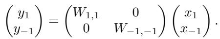
In the equation above:

• \(W_{1,1}\) maps invariant inputs to invariant outputs.
• \(W_{-1,-1}\) maps (-1)-equivariant inputs to (-1)-equivariant outputs.
• The off-diagonal blocks (which would map invariant to equivariant or vice versa) must be zero.

Why This Saves Compute

This is where the magic happens. A standard matrix multiplication of size \(N \times N\) requires roughly \(N^2\) operations.

By splitting the features evenly (half invariant, half equivariant) and forcing the off-diagonals to zero, we perform two smaller matrix multiplications of size \((N/2) \times (N/2)\).

We have just cut the number of FLOPs in half.

This result stems from Schur’s Lemma, a fundamental theorem in representation theory. It essentially says that linear maps between different types of irreducible representations (irreps) must be zero. By parametrizing the network in terms of these irreps (symmetric and antisymmetric features), the computational savings come naturally.

Building the Architecture

How do we implement this in practice? We can’t just apply this logic to a black box; we need to adapt the specific layers of modern vision architectures.

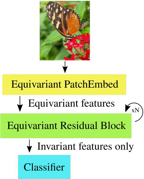
The schematic above illustrates the “Geometric Deep Learning Blueprint.” We start with an equivariant embedding, process features through equivariant blocks, and finally collapse them into invariant features for the classifier (since the final label “Cat” shouldn’t flip).

1. The Patch Embedding

Everything starts with the input image. To enter our equivariant pipeline, we need to convert the raw RGB pixels into our two feature types: invariant and (-1)-equivariant.

We do this using a modified Patch Embedding layer.

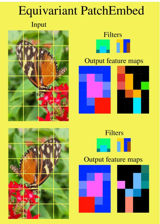
As shown in Figure 2, the authors enforce constraints on the convolutional filters:

• Symmetric Filters: Produce invariant features.
• Antisymmetric Filters: Produce (-1)-equivariant features (they flip sign when the underlying patch is flipped).

This creates the initial split of the feature stream.

2. Non-Linearities (GELU)

Linear layers are easy to block-diagonalize, but neural networks need non-linearities like GELU or ReLU to function. How do you apply a non-linearity to a feature that is supposed to flip signs? If you just apply ReLU to a negative number, it becomes zero, destroying the symmetry information.

The authors solve this by transforming the features. They temporarily mix the invariant (\(x_1\)) and equivariant (\(x_{-1}\)) parts to move into a “spatial” domain (\(s\) and \(t\)), apply the non-linearity there, and then transform back.

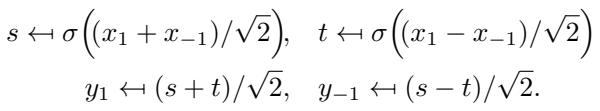
While this looks slightly more complex than a standard GELU(x), the computational cost is negligible compared to the savings gained in the linear layers.

3. Attention

For Vision Transformers (ViT), the Self-Attention mechanism is critical. The authors adapt this by splitting Queries (\(q\)) and Keys (\(k\)) into their symmetric and antisymmetric parts.

The dot product (which determines attention scores) becomes:

Notice the term \((-q_{i,-1}) \cdot (-k_{j,-1})\). Because both terms flip signs, the negatives cancel out, and the resulting attention score \(a_{ij}\) remains invariant. This ensures that the attention map describes the relationship between patches regardless of the image orientation.

Adapting Modern Backbones

The authors didn’t just propose a theoretical module; they adapted three of the most popular computer vision architectures: ResMLP, ViT, and ConvNeXt.

ResMLP

ResMLP is an architecture that consists almost entirely of linear layers (MLPs). Since the authors’ method cuts linear layer compute by 50%, ResMLP benefits massively.

The residual block structure is modified to respect the feature splits:

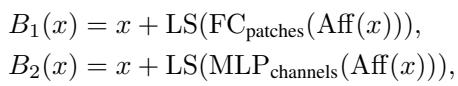
Because ResMLP is so dense-computation heavy, the “Flopping” technique results in the most dramatic speedups here.

ConvNeXt

ConvNeXt is a modernized Convolutional Network. The heavy lifting in ConvNeXt is done by depthwise convolutions followed by \(1 \times 1\) convolutions (which are mathematically identical to linear layers).

The \(1 \times 1\) convolutions get the block-diagonal treatment (50% savings). For the depthwise spatial convolutions, the authors alternate between symmetric and antisymmetric kernels.

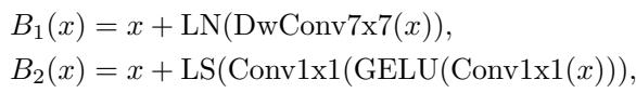
While they didn’t write custom GPU kernels to fully optimize the depthwise layer (using Winograd algorithms for symmetry), the standard implementation still benefits significantly from the reduction in the pointwise layers.

Experiments: Does it Work?

The theoretical reduction in FLOPs is clear, but does it translate to performance? Sometimes, restricting a network to be equivariant forces it to learn “worse” features, dropping accuracy.

The authors tested their equivariant models (\(\mathcal{E}\)) against standard baselines on ImageNet-1K.

FLOPs vs. Parameters

First, let’s look at the scaling properties.

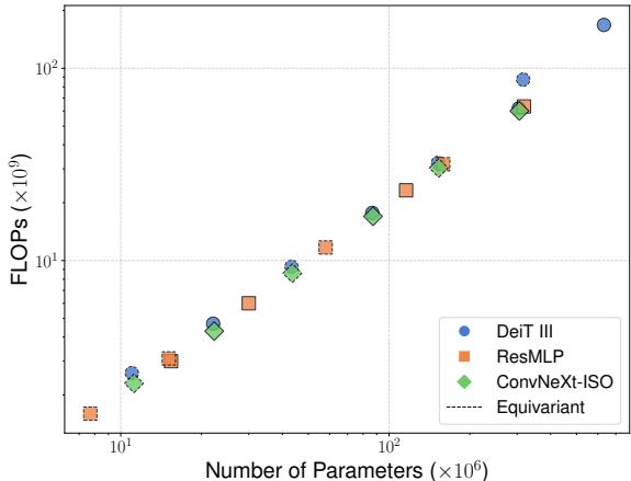
In standard networks, FLOPs and parameters usually scale together linearly. The dashed line in Figure 4 represents the Equivariant models. You can see they occupy a unique space in the efficiency landscape, maintaining the parameter count of larger models while drastically reducing the compute requirements.

Accuracy vs. Compute

The most critical chart for any efficiency paper is the trade-off between Accuracy and Compute (FLOPs).

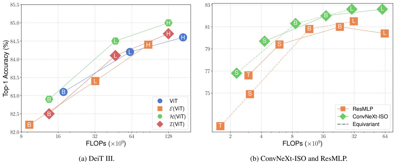
In Figure 5, look at the plot for ConvNeXt-ISO and ResMLP (bottom). The Equivariant models (black dotted line) consistently appear to the left of the baseline models for the same accuracy. This means they achieve comparable results with significantly less computation.

For DeiT III (ViT) (top chart), the results are also compelling. The equivariant versions (\(\mathcal{E}(ViT)\)) achieve accuracy very close to the baselines but at a fraction of the FLOPs. For example, \(\mathcal{E}(ViT-L)\) (Large) runs with roughly the compute budget of a standard ViT-B (Base) but achieves higher accuracy.

Throughput (Real Speed)

FLOPs are a theoretical measure. Real-world speed (images per second) depends on memory bandwidth and GPU kernel implementation.

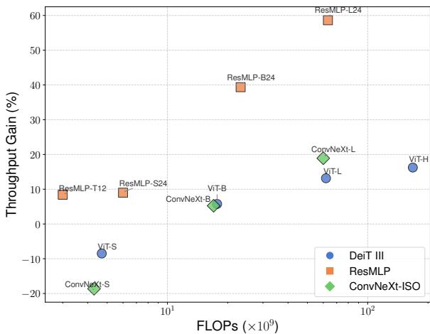
Figure 6 shows the “Throughput Gain.”

• ResMLP (Orange): Shows massive gains (up to 60% faster). Since ResMLP is dominated by big matrix multiplications, the block-diagonalization pays off immediately.
• ViT and ConvNeXt: The gains increase as the model size grows. For small models (Small/Tiny), the overhead of managing the feature splits slightly outweighs the math benefits. But as models scale up (Large/Huge), the matrix multiplications dominate, and the equivariant models run significantly faster than their standard counterparts.

Key Takeaways

The “Bitter Lesson” suggests we should stop trying to be clever and just scale compute. This paper offers a “sweet” counter-argument: being clever about symmetry allows us to scale compute more effectively.

Here is the summary of what “Flopping for FLOPs” achieves:

1. Block-Diagonal Efficiency: By decomposing features into invariant and (-1)-equivariant types, dense linear layers are split into two smaller blocks, halving the FLOPs.
2. Universal Applicability: This isn’t just for niche architectures. It works on ViTs, MLPs, and ConvNets.
3. Scalability: The efficiency gains get better as the models get bigger. This makes it a promising technique for the era of Foundation Models.
4. No “Symmetry Tax”: Unlike previous equivariant approaches that increased compute density, this method reduces it while maintaining comparable accuracy.

By hard-coding the knowledge that “a flipped image is still the same image,” we don’t just save the model from having to learn that fact—we save the GPU from having to compute it.