Introduction

Diffusion models have fundamentally changed the landscape of generative AI. From DALL-E to Stable Diffusion, the ability to generate high-fidelity images from Gaussian noise is nothing short of magical. However, standard diffusion models have a specific limitation: they generally assume a transition from a standard Gaussian distribution (pure noise) to a data distribution (an image).

But what if you don’t want to start from noise? What if you want to transition from one specific distribution to another? Consider image restoration: you want to move from a “Low-Quality” (LQ) distribution—blurry, rainy, or masked images—to a “High-Quality” (HQ) distribution. This requires a Diffusion Bridge.

Existing methods attempt to solve this by creating a bridge between two fixed endpoints using a mathematical technique called Doob’s h-transform. While mathematically sound, these methods often force the model to hit the target so aggressively that the generated images suffer from unnatural artifacts, blurring, or over-smoothing.

Enter UniDB, a novel framework presented in the paper “UniDB: A Unified Diffusion Bridge Framework via Stochastic Optimal Control.” This research reimagines the diffusion bridge not just as a statistical transformation, but as a Stochastic Optimal Control (SOC) problem. By doing so, the authors not only unify existing methods under one theoretical roof but also introduce a “tunable” penalty coefficient that significantly improves image quality.

In this deep dive, we will explore how UniDB uses control theory to fix the flaws of previous diffusion bridges, unifying the mathematics of image restoration.

Background: The Diffusion Bridge Problem

To understand UniDB, we first need to understand the limitations it addresses. Standard diffusion models rely on a forward process that adds noise and a reverse process that removes it.

The equation governing the forward process is typically a Stochastic Differential Equation (SDE):

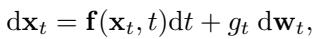
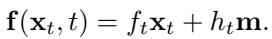
Here, \(\mathbf{f}\) is the drift (the deterministic push) and \(g_t\) is the diffusion (the random noise). In many standard models, the drift is linear:

The Limitation of Doob’s h-Transform

When we want to bridge two specific distributions (e.g., converting a blurry photo to a sharp one), we need to condition the diffusion process so that it starts at \(\mathbf{x}_0\) and guarantees arrival at \(\mathbf{x}_T\).

Historically, researchers used Doob’s h-transform. This technique modifies the drift of the SDE to force the path to hit a specific terminal point \(\mathbf{x}_T\). The modified forward process looks like this:

The term \(\mathbf{h}(\mathbf{x}_t, t, \mathbf{x}_T, T)\) is an extra “force” added to the drift to ensure the particle lands exactly on the target. While this works in theory, the authors of UniDB identify a critical flaw: it is too rigid.

By forcing the trajectory to match the endpoint exactly (a hard constraint), the model often has to make “unnatural” moves in the state space, leading to local blurring and distortion. It lacks the flexibility to trade off a tiny bit of endpoint accuracy for a much smoother, more realistic image trajectory.

The Core Method: UniDB via Stochastic Optimal Control

The primary contribution of UniDB is shifting the perspective from simple probability transformation to Stochastic Optimal Control (SOC).

In SOC, we act as a “controller.” We want to guide a system (the image generation process) from a start state to a goal state. However, we have to pay a “cost” for applying control (energy), and we pay a “penalty” if we miss the target.

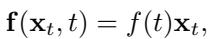
Visualizing the Difference

The figure below perfectly illustrates the intuition behind UniDB compared to the traditional Doob’s approach.

In the green box (Doob’s \(h\)-transform), the path is forced. In the red box (UniDB), the path is optimized. You can see in the sample images at the bottom of the figure that the UniDB output (Red) recovers fine textures (like the microphone mesh or the grass) that the Doob’s method (Green) blurs out.

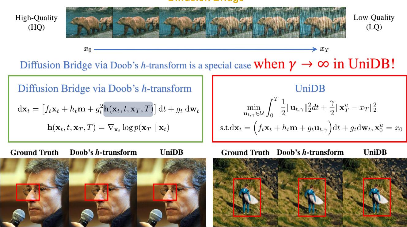
Formulating the Optimization Problem

UniDB defines the diffusion bridge as an optimization problem. We want to find a control function \(\mathbf{u}_{t, \gamma}\) that minimizes a specific cost function:

Let’s break down this equation, as it is the heart of the paper:

1. The Integral Term (\(\int \frac{1}{2} \|\mathbf{u}\|^2 dt\)): This represents the “Control Cost.” It effectively penalizes the model for making wild, high-energy changes to the image trajectory. We want the path to be smooth and “easy” to traverse.
2. The Terminal Term (\(\frac{\gamma}{2} \|\mathbf{x}_T^u - x_T\|^2\)): This is the “Terminal Penalty.” It penalizes the model based on how far the final generated image \(\mathbf{x}_T^u\) is from the target target ground truth \(\mathbf{x}_T\).
3. The Coefficient \(\gamma\): This is the magic number. It controls the trade-off. A high \(\gamma\) means “Hit the target at all costs!” A low \(\gamma\) means “Focus on a smooth path, even if you miss the target slightly.”

The system is subject to the linear SDE:

This setup allows the authors to derive a closed-form solution for the optimal controller. Because the system is linear and the costs are quadratic (a Linear-Quadratic-Gaussian control problem), we can solve it analytically.

The Optimal Controller

Through the application of the Pontryagin Maximum Principle (a fundamental theorem in optimal control), the authors derive the exact formula for the optimal control input \(\mathbf{u}^*_{t, \gamma}\):

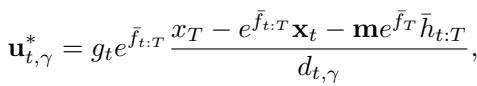
This equation might look intimidating, but it tells a story. The optimal push (\(\mathbf{u}^*\)) depends on the current state \(\mathbf{x}_t\), the target \(\mathbf{x}_T\), and the parameter \(\gamma\) (hidden inside the term \(d_{t, \gamma}\)).

The “Aha!” Moment: Unifying the Theory

Here is the most significant theoretical contribution of the paper. The authors prove that the traditional method (Doob’s \(h\)-transform) is actually just a special case of UniDB.

Specifically, if you take the UniDB framework and let the penalty coefficient \(\gamma\) go to infinity (\(\gamma \to \infty\)), the UniDB controller becomes mathematically identical to Doob’s \(h\)-transform.

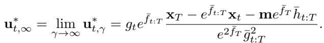
This explains why previous methods had quality issues. By implicitly setting \(\gamma = \infty\), previous models were solving an optimization problem where the “control cost” (smoothness) was ignored in favor of infinite strictness on the endpoint. This forces the SDE to take “expensive” (unnatural) paths to satisfy the hard constraint, resulting in the artifacts seen in previous figures.

The authors formally propose that the optimal controller with a finite \(\gamma\) yields a lower total cost (better balance of smoothness and accuracy) than the infinite case:

By treating \(\gamma\) as a hyperparameter rather than a fixed infinite value, UniDB gains the flexibility to generate higher-quality images.

Implementation: UniDB-GOU

To test this theory, the authors apply UniDB to the Generalized Ornstein-Uhlenbeck (GOU) process. GOUB (GOU Bridge) is a state-of-the-art method for image restoration. By upgrading GOUB with the UniDB framework, they create UniDB-GOU.

The forward SDE for UniDB-GOU looks like this:

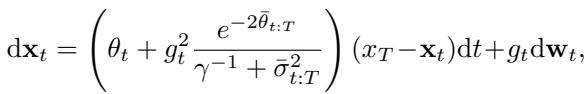
Notice the term involving \(\gamma^{-1}\). If \(\gamma \to \infty\), then \(\gamma^{-1} \to 0\), and this equation collapses back into the standard GOUB equation. But with a finite \(\gamma\), the drift is modulated, preventing the “force” from becoming too extreme near the endpoint.

The Training Objective

How do we actually train a neural network to learn this? The authors derive a loss function based on the transition probabilities. The network predicts the score (gradient of the log-density), and the loss measures the difference between the “posterior mean” (where the math says we should be) and the “predicted mean” (where the network says we are).

The training objective is formulated as:

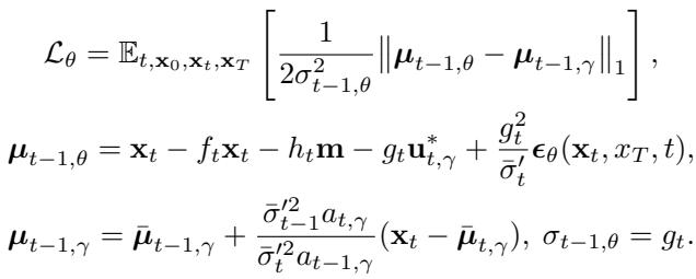
This looks complex, but functionally, it is very similar to standard diffusion training, just with modified coefficients (\(a_{t, \gamma}\) and \(\bar{\mu}_{t, \gamma}\)) that account for the control parameter \(\gamma\). This means UniDB can be integrated into existing codebases with minimal code modifications. You simply swap out the coefficient formulas.

Experiments and Results

The researchers evaluated UniDB on three major image restoration tasks:

1. Image Super-Resolution (Making small images 4x larger).
2. Image Deraining (Removing rain streaks).
3. Image Inpainting (Filling in missing parts of an image).

Quantitative Analysis

The results, summarized in the table below, show that UniDB consistently outperforms baselines like GOUB, IR-SDE, and DDRM.

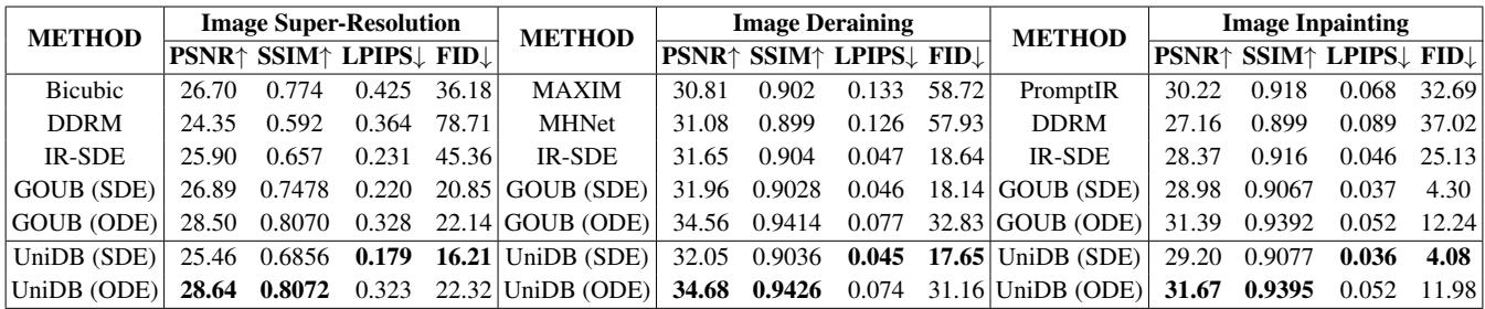
Key metrics to look at:

• PSNR/SSIM: Higher is better. These measure signal fidelity. UniDB achieves top scores here.
• LPIPS/FID: Lower is better. These measure perceptual quality (how “real” the image looks to a human). UniDB shows significant drops in FID, indicating much more realistic textures.

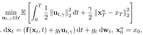
Visual Analysis

Numbers are great, but in image generation, the eyes have the final say.

Super-Resolution (4x)

In the figure below, compare the “GOUB” column with the “UniDB” column against the Ground Truth (GT).

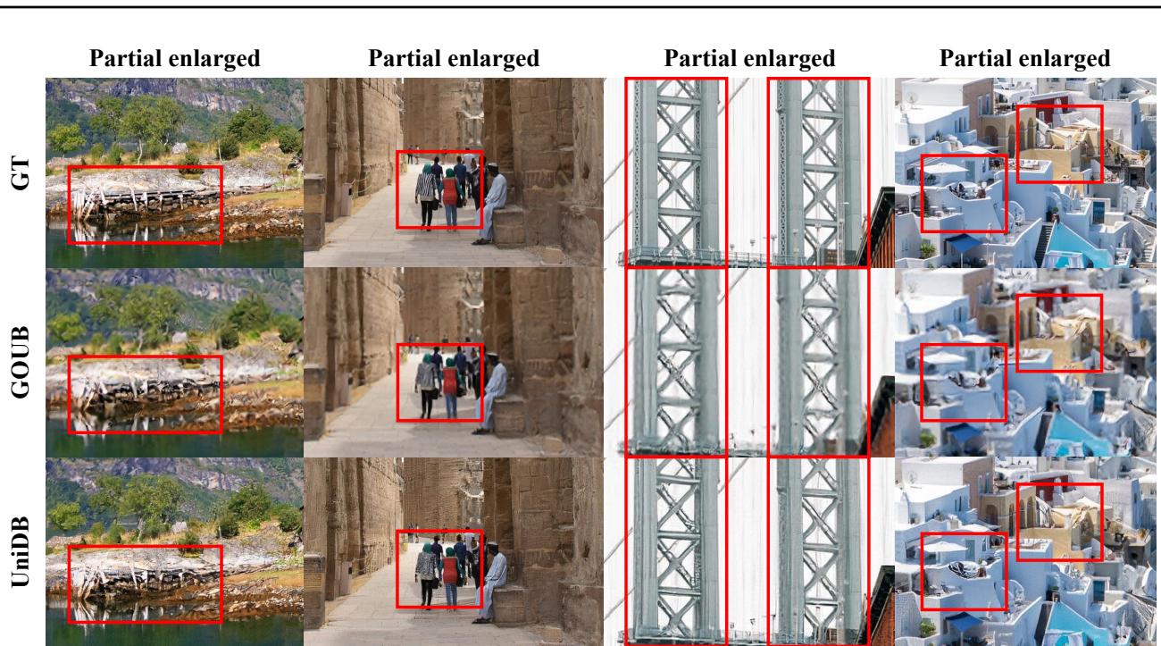
Look closely at the red zoomed-in boxes. GOUB often leaves the textures slightly muddy or overly smoothed. UniDB recovers sharp edges and specific textures that align much better with the Ground Truth.

Deraining and Inpainting

The same trend holds for removing rain and filling in faces.

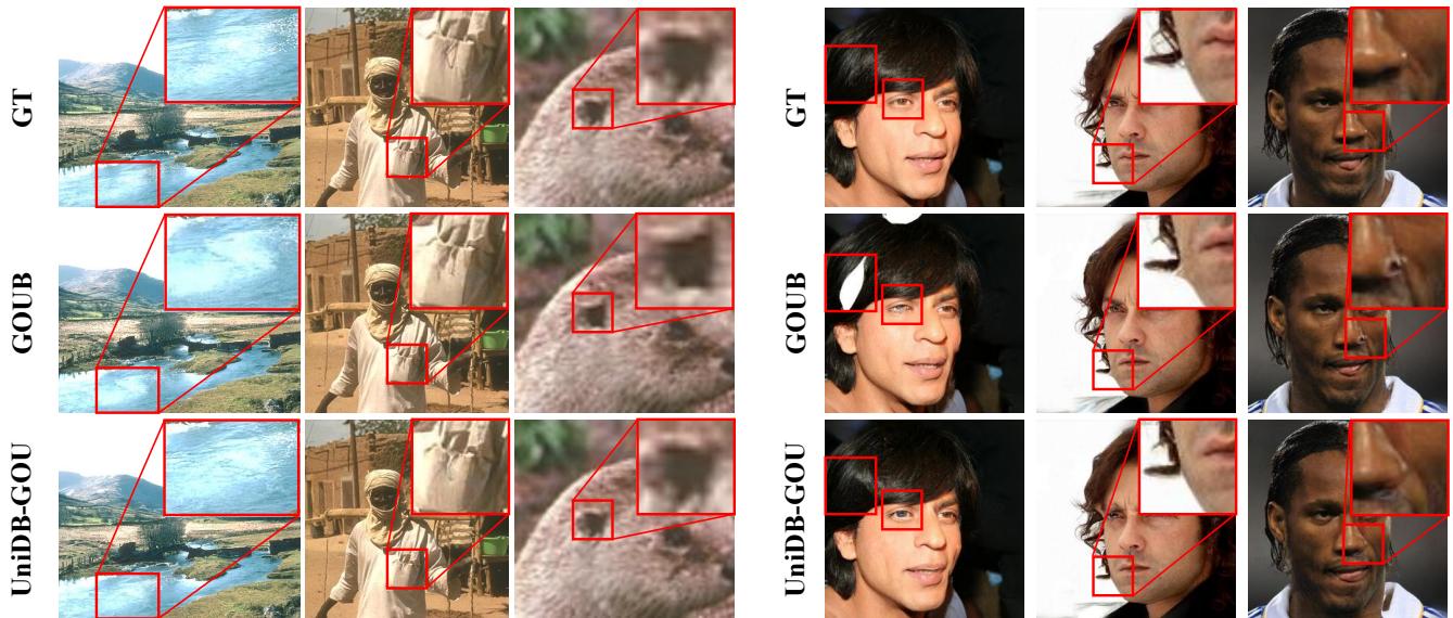
In the inpainting task (right side), look at the facial features. UniDB generates eyes and noses that are structurally consistent and sharp, whereas previous methods sometimes produce “dream-like” blurry features.

The Gamma Ablation Study

One of the most interesting parts of the paper is the analysis of \(\gamma\). Since \(\gamma\) controls the balance between “smoothness” and “accuracy,” there should be a “sweet spot.”

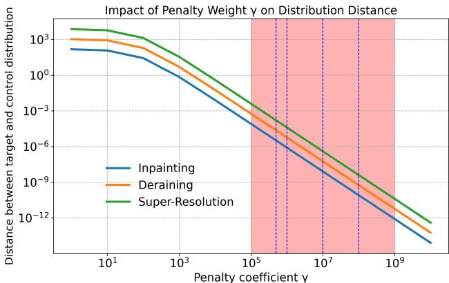
This graph plots the distance between the generated distribution and the target distribution.

• As \(\gamma\) increases (moving right), the distance decreases (the model hits the target more accurately).
• However, the authors found that beyond a certain point (around \(10^7\) or \(10^8\)), the perceptual quality (FID) starts to degrade, even if the math says the distance is smaller.
• The “sweet spot” (shaded red region) represents a finite \(\gamma\) where the model is accurate enough but retains the freedom to generate natural, high-frequency details.

Conclusion and Implications

UniDB represents a significant step forward in the theoretical understanding of diffusion bridges. By reframing the problem through the lens of Stochastic Optimal Control, the authors have:

1. Unified the field: Showing that Doob’s \(h\)-transform and various other bridge models (VP, VE, GOU) are all special cases of a single control framework.
2. Identified the root cause of artifacts: Attributing blurring and distortion to the implicit “infinite penalty” in previous methods.
3. Provided a practical solution: Introducing the tunable \(\gamma\) parameter, which improves results on super-resolution, inpainting, and deraining with minimal code changes.

For students and researchers, UniDB offers a powerful lesson: sometimes, relaxing a hard constraint (like exact endpoint matching) allows for a globally better solution. By thinking like a pilot trying to fly smoothly rather than just a mathematician trying to force a point match, we can build better generative models.

The code for UniDB is available for those looking to experiment with this new framework, promising a new standard for conditional image generation tasks.