](https://deep-paper.org/en/paper/2502.06768/images/cover.png)
If you have used ChatGPT or any modern Large Language Model (LLM), you have interacted with an Autoregressive Model (ARM). These models generate text in a very specific way: token by token, from left to right. They are incredibly successful, but they are also rigid. They must decide what comes next based entirely on what came before.
But what if the “next” token isn’t the easiest one to predict? What if the end of the sentence is easier to guess than the middle?
Enter Masked Diffusion Models (MDMs). Unlike their autoregressive cousins, MDMs can generate tokens in any order. They work by gradually filling in the blanks (unmasking) of a corrupted sequence.
For a long time, the consensus was that MDMs were interesting but generally inferior to ARMs for language modeling. They were harder to train and often achieved worse perplexity. However, a fascinating new paper titled “Train for the Worst, Plan for the Best” flips this narrative. The researchers propose that the very thing that makes MDMs hard to train—the lack of a fixed order—is exactly what makes them superior reasoners at inference time.
In this post, we will dive deep into this paper. We will explore why MDMs face such a brutal training landscape, how this complexity allows them to “plan” their generation strategies, and how a simple change in inference allows them to crush logic puzzles like Sudoku, significantly outperforming standard autoregressive models.
1. Background: The Tale of Two Models
To understand the contribution of this paper, we first need to distinguish between the two dominant paradigms in discrete generative modeling.
The Rigid Expert: Autoregressive Models (ARMs)
ARMs operate on a simple principle: Order Matters. Specifically, the left-to-right order. When an ARM is trained, it learns to predict the next token \(x_i\) given the history \(x_{0}, \dots, x_{i-1}\).
Mathematically, this decomposes the probability of a sequence \(x\) into a product of conditional probabilities:
\[ p(x) = \prod_{i=1}^{L} p(x_i | x_{The Flexible Generalist: Masked Diffusion Models (MDMs)
MDMs take a different approach. They are trained to reverse a noise process. In the discrete world (like text), “noise” usually means masking tokens.
The Forward Process:
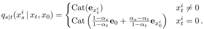
We start with clean data \(x_0\). We gradually corrupt it by replacing tokens with a special [MASK] token (denoted as 0). At time \(t=0\), we have the original sentence. At time \(t=1\), we have a sequence of pure masks.

Here, \(\alpha_t\) controls the noise schedule. As \(t\) goes from 0 to 1, the probability of a token being masked increases.
The Reverse Process: The goal of the MDM is to learn the reverse operation: given a partially masked sequence \(x_t\), predict the original values of the masked tokens.
The crucial difference here is combinatorics. An ARM sees a sequence of length \(L\) and learns \(L\) transitions. An MDM, however, might see any combination of masked and unmasked tokens. It effectively has to learn how to predict any subset of tokens given any other subset.
2. Train for the Worst: The Burden of Complexity
The authors of the paper start by investigating a burning question: Why are MDMs harder to train than ARMs?
It turns out that the flexibility of MDMs comes at a steep price during training. Because an MDM doesn’t know which order it will be asked to generate data in, it must learn to handle every order.
Order-Agnostic vs. Order-Aware
The paper formalizes this distinction using the concept of \(\pi\)-learners (permutation learners).
- ARM: Uses a fixed identity permutation (left-to-right). It is Order-Aware.
- MDM: Effectively averages over all possible permutations. It is Order-Agnostic.
The researchers prove that Order-Agnostic training is computationally intractable for many data distributions compared to Order-Aware training.
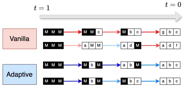
As shown in the top half of Figure 1 above, training an MDM is like forcing a student to learn to solve a math proof starting from the middle, the end, or the beginning randomly. Some of those sub-problems are incredibly hard.
The “Latents-and-Observations” Theory
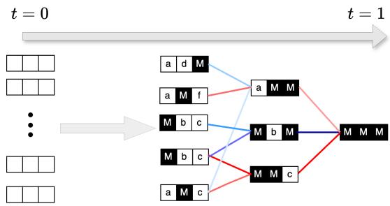
To prove this mathematically, the authors introduce the Latents-and-Observations (L&O) distribution model. Imagine a dataset generated in two steps:
- Latents (Hidden Seeds): First, random “seed” numbers are generated.
- Observations (The Result): Then, visible numbers are calculated based on those seeds using a function (e.g., a hash or a logic rule).
The Asymmetry:
- If you generate in the “natural” order (Seeds \(\rightarrow\) Observations), the task is easy. You just run the function.
- If you generate in the “wrong” order (Observations \(\rightarrow\) Seeds), you have to invert the function. If the function is complex (like a hash), this is computationally impossible.
ARMs, if trained in the natural order, only face the easy task. MDMs, because they train on random masks, will frequently encounter the “wrong” order sub-problems (trying to guess the seed from the observation).
Empirical Evidence
The authors validated this theory not just with math, but with real models. They compared the “hardness” (likelihood) of learning text in a fixed order (ARM) versus random orders (MDM).
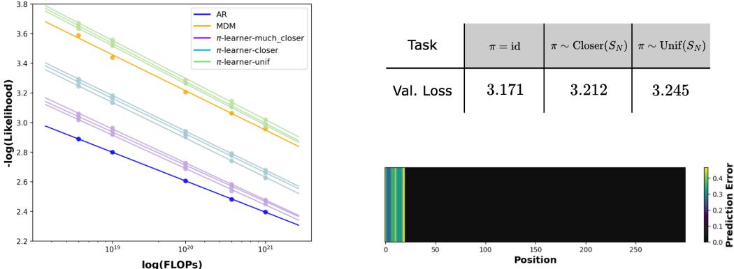
In Figure 2 (Left), we see the cost of this complexity. The orange line (MDM) consistently has a worse likelihood (higher negative log-likelihood) than the blue line (ARM) for the same compute budget (FLOPs).
The heatmap in Figure 2 (Right) is even more revealing. It shows “Task Error Imbalance.” The dark regions represent easy tasks (observation positions), while the light regions represent hard tasks (latent positions). The MDM struggles significantly with the “hard” parts of the distribution—the parts that ARMs simply skip by virtue of their fixed ordering.
3. Plan for the Best: The Power of Adaptive Inference
So far, things look grim for Masked Diffusion. They are forced to learn intractable problems and suffer in performance metrics. Why bother?
Here lies the paper’s second, transformative insight: You don’t have to use the random order during inference.
While the MDM was forced to learn the hard problems during training, it also learned the easy ones. At inference time, we have the freedom to choose the generation path. We can “plan” our route to avoid the intractable cliffs and stick to the easy valleys.
Breaking Free from Randomness
Standard (Vanilla) MDM inference mimics the training noise process: it unmasks tokens randomly. This is inefficient because it risks asking the model to solve a hard sub-problem (like guessing a seed) when it isn’t ready.
Adaptive Inference changes the game. Instead of picking a random set of tokens to unmask, we ask the model: “Which tokens are you most confident about?”
As visualized above, Vanilla inference might take a path that requires guessing a hard token early (e.g., M \(\rightarrow\) b). Adaptive inference steers the generation path through the easiest transitions first.
The Strategies: Top Probability vs. Margin
The authors propose using an Oracle \(\mathcal{F}(\theta, x_t)\) to select which tokens to unmask next. They test two primary strategies:
Top Probability: Unmask the token where the model assigns the highest probability to a single value.
\[ \mathcal{F} = \text{Top } K (\max_j p_\theta(x^i=j | x_t)) \]Problem: Sometimes the model is “confidently wrong” or splits probability high between two very likely options (e.g., “The cat sat on the [mat/hat]”).
Top Probability Margin (The Winner): Unmask the token where the gap between the best guess and the second-best guess is largest.
\[ \mathcal{F}(\theta, x_t) = \text{Top } K \left( |p_\theta(x^i = j_1 | x_t) - p_\theta(x^i = j_2 | x_t)| + \epsilon \right) \]
This strategy prefers tokens where the model is unambiguous. If the model thinks it’s 50/50 between “mat” and “hat”, the margin is 0, so it waits. If it thinks it’s 99% “mat” and 1% “hat”, the margin is high, so it unmasks it.
4. Experimental Results: Crushing Logic Puzzles
The theoretical benefits of Adaptive Inference are substantial, but the empirical results on logic puzzles are staggering.
The authors tested the models on Sudoku and Zebra Puzzles (Einstein riddles). These are perfect test beds because they have a “logical” order of solution that is rarely left-to-right. In Sudoku, you solve the cell with the fewest possibilities first, regardless of where it sits on the grid.
The Sudoku Showdown
The authors compared three contenders:
- ARM (Standard): Trained left-to-right.
- ARM (Teacher Forced): Explicitly trained with the optimal solving order (a huge advantage).
- MDM (Adaptive): Trained normally (randomly), but using Top Probability Margin at inference.
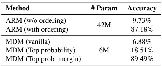
Note: The table above (Table 2 in the paper) shows the accuracy jump.
The results were shocking:
- Vanilla MDM: < 7% accuracy. (Random guessing is bad for logic).
- ARM (Standard): ~10% accuracy. (Left-to-right is terrible for Sudoku).
- ARM (Optimal Order): 87.18% accuracy. (Knowing the order helps).
- MDM (Adaptive Margin): 89.49% accuracy.
Key Takeaway: The MDM, which was never explicitly taught the rules of Sudoku or the correct order of operations, figured out a better solving order on the fly than an ARM that was explicitly supervised with the correct order.
Zebra Puzzles
The results held for Zebra puzzles as well, which require complex relational reasoning.
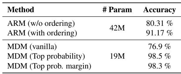
As shown in Table 3, the MDM with adaptive inference reached 98.3% accuracy, surpassing the best ARM baseline (91.17%).
Generalizing to Text and Math
While logic puzzles are the highlight, the authors also showed that this technique applies to standard Large Language Models. They applied adaptive inference to LLaDa 8B, a large Masked Diffusion Model.
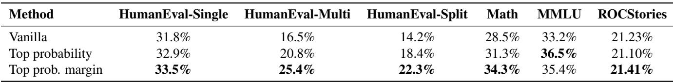
On difficult reasoning tasks like HumanEval (Coding) and GSM8K (Math), the Adaptive “Top Probability Margin” strategy consistently outperformed Vanilla inference. For example, on HumanEval-Multi, performance jumped from 16.5% (Vanilla) to 25.4% (Margin).
We also see this benefit in pure generation metrics.
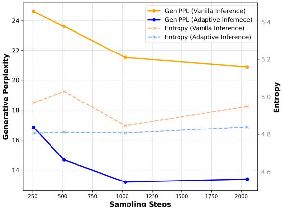
Figure 3 shows that Adaptive Inference (Blue line) dramatically lowers the perplexity (a measure of “surprise” or error) compared to Vanilla inference (Orange line), effectively matching the text quality of autoregressive models while maintaining diversity.
5. Conclusion: The Future is Non-Sequential
The paper “Train for the Worst, Plan for the Best” offers a resolution to the complexity-flexibility paradox of Masked Diffusion Models.
- Training Complexity: Yes, MDMs face a harder training task than ARMs because they must learn to predict variables from observations (the “hard” direction) rather than just generating variables sequentially.
- Inference Flexibility: However, this exhaustive training gives them a “holistic” understanding of the data. They know the connections between all parts of the sequence.
- Adaptive Power: By using strategies like Top Probability Margin, we can dynamically construct the optimal generation path for every specific input.
The most profound finding is that MDMs can discover optimal reasoning paths without supervision. In Sudoku, the model naturally learned to fill in the easiest numbers first, deriving a strategy purely from the statistical properties of its own uncertainty.
This suggests that for tasks requiring planning, logic, and non-linear reasoning, the dominance of left-to-right Autoregressive Models may be coming to an end. By training for the worst-case masking scenarios, MDMs are uniquely prepared to plan for the best possible solutions.