](https://deep-paper.org/en/paper/2502.07827/images/cover.png)
Introduction
In the current landscape of Deep Learning, we are witnessing a massive tug-of-war between two fundamental properties: parallelization and expressivity.
On one side, we have Transformers and State-Space Models (SSMs) like Mamba. These architectures dominate because they are highly parallelizable during training. You can feed them a sequence of text, and they process all tokens simultaneously using GPUs. However, there is a catch. Theoretically, these models belong to a complexity class (specifically \(TC^0\)) that cannot fully solve inherently sequential problems, such as tracking state in a finite state machine (FSM) or solving complex parity problems. They suffer from a “depth” limit.
On the other side, we have classical Recurrent Neural Networks (RNNs). RNNs process data sequentially, updating a hidden state step-by-step. This makes them incredibly expressive for state-tracking problems—they can theoretically model any algorithm that an FSM can. But, they are painfully slow to train because you cannot parallelize the sequential dependency (step \(t\) waits for step \(t-1\)).
This leads to a fundamental question: Must we sacrifice the ability to reason sequentially to gain training speed?
A new research paper, Implicit Language Models are RNNs: Balancing Parallelization and Expressivity, suggests the answer is no. The researchers propose Implicit SSMs. By iterating a transformation until it converges to a “fixed point,” these models behave like parallelizable Transformers during training but act like infinitely deep, non-linear RNNs during inference.
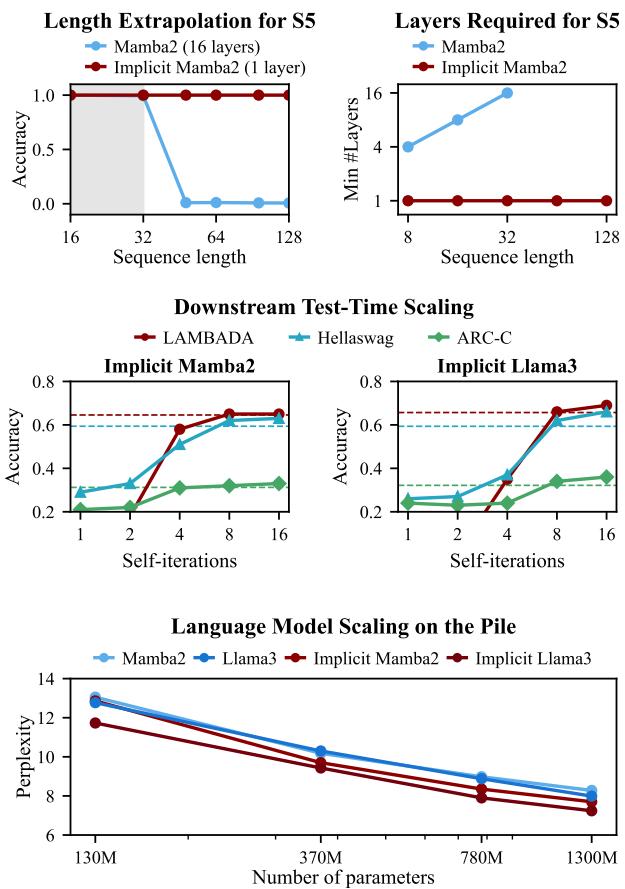
As shown in the figure below, the results are striking. While standard models like Mamba2 fail to generalize to longer sequences or solve hard logic puzzles (\(S_5\)), Implicit Mamba2 maintains accuracy regardless of sequence length.
In this post, we will tear down this paper to understand how Implicit Models work, the mathematics behind their “infinite” depth, and how they were scaled to train Large Language Models (LLMs) with 1.3 billion parameters.
Background: The Illusion of State
To understand why Implicit Models are necessary, we first need to understand the limitations of current architectures.
The Limitation of Explicit Models
Most modern language models are “explicit.” This means they consists of a fixed stack of layers (e.g., 32 layers in Llama-2-7B). When a token passes through the network, it undergoes a finite, predetermined number of non-linear transformations.
Recent theoretical work has shown that this finite depth creates a ceiling on computational power. Specifically, Transformers and SSMs struggle with state tracking. Imagine a problem where you need to track the location of an object as it is moved between boxes A, B, and C over a sequence of 100 moves. If the logic requires updating a state based strictly on the previous state, standard parallel models often fail or require a number of layers that scales with the input length.
Classical RNNs don’t have this problem because their state evolves sequentially. However, as noted, we stopped using them because they don’t scale on modern hardware.
Deep Equilibrium Models (DEQs)
The researchers drew inspiration from Deep Equilibrium Models (DEQs). Unlike a standard network where \(y = f_3(f_2(f_1(x)))\), a DEQ defines its output implicitly. It asks: “What is the vector \(z^*\) such that if I run it through the network again, it doesn’t change?”
Mathematically, we look for the fixed point \(z^*\) of a function \(F_\theta\):
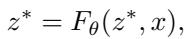
Finding this \(z^*\) usually involves iterating the function over and over (self-iteration) until the values stabilize. This implies that the “effective depth” of the network adapts to the difficulty of the input. Easy inputs converge fast; hard inputs take longer.
The Core Method: Implicit SSMs
The researchers propose merging the architecture of State-Space Models (specifically Mamba2) with the infinite-depth philosophy of DEQs.
The Architecture
In a standard SSM, a hidden state \(h_t\) is updated using a linear recurrence: \(h_t = \Lambda h_{t-1} + u_t\). This linearity is what allows SSMs to be parallelized (using algorithms like parallel scan). But it is also what limits their expressivity.
The Implicit SSM modifies this by introducing a “depth” variable \(s\). We process the sequence over time \(t\), but at each timestep, we also iterate “vertically” through depth \(s\) until convergence.
The update rule becomes a fixed-point iteration:
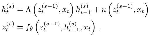
Here:
- \(t\) is the time step (sequence position).
- \(s\) is the iteration step (depth).
- \(h_t^{(s)}\) is the hidden state.
- \(z_t^{(s)}\) is the layer output (or “thought” vector).
Notice that the transition matrices \(\Lambda\) and inputs \(u\) now depend on the previous iteration’s output \(z_t^{(s-1)}\). This couples the state evolution to the depth iteration.
Two Modes of Operation: The “Duality”
One of the paper’s most significant contributions is defining two distinct ways to compute these fixed points. This duality allows the model to be efficient in different contexts.
1. Simultaneous Mode (Best for Training) In this mode, we iterate the entire sequence at once. We update all tokens (\(t=1\) to \(T\)) for iteration \(s=1\), then all tokens for \(s=2\), and so on. Because the underlying SSM core is parallelizable, each iteration \(s\) is fast. This allows the model to be trained efficiently on GPUs.
2. Sequential Mode (Best for Inference) In this mode, we solve the fixed point for token \(t=1\) completely (looping \(s\) until convergence), then pass the final state to \(t=2\), solve for \(t=2\), and so on. This behaves exactly like an RNN.
The image below visualizes this beautiful duality. The “Simultaneous” mode (A) allows trajectories to interact during convergence, while the “Sequential” mode (B) processes one token at a time.
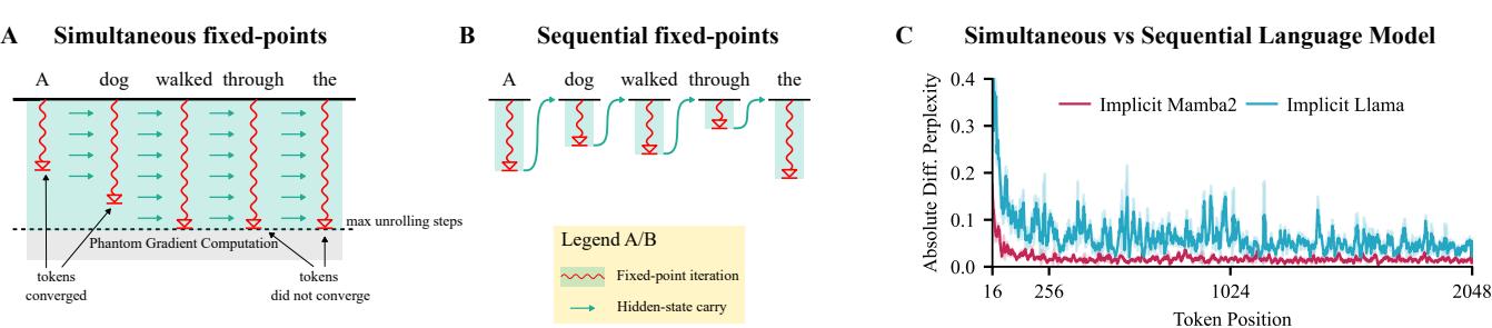
The graph in Panel C confirms that both modes produce nearly identical results (low perplexity difference), proving they are functionally equivalent.
Theoretical Proof: It Is an RNN
Why go through this trouble? The researchers provide a theorem proving that at convergence (when \(s \to \infty\)), the linear limitations of the SSM vanish.
In the limit, the fixed point variables \(h^*\) and \(z^*\) satisfy:
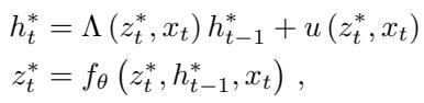
The researchers derived the Jacobian (the rate of change) of the state \(h_t^*\) with respect to the previous state \(h_{t-1}^*\). In a standard SSM, this Jacobian is diagonal and linear. In an Implicit SSM, the Jacobian becomes:
This equation shows that the transition is non-linear and non-diagonal. The state evolution depends on complex interactions between the hidden state and the input. In layman’s terms: The Implicit SSM has theoretically transformed itself into a non-linear RNN, gaining the computational power to solve complex state-tracking problems that baffle standard Transformers.
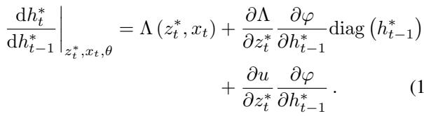
We can visualize this non-linearity. The heatmap below compares the gradients derived via automatic differentiation (Autograd) vs. the theoretical formula above. The presence of off-diagonal elements (the colorful patterns) confirms the model is learning complex state dependencies.
Training with Phantom Gradients
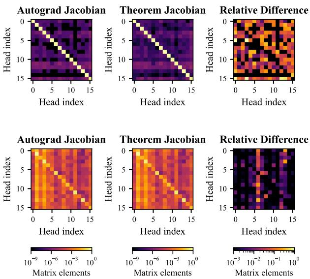
Training a model with “infinite” depth sounds memory-intensive. If you unroll a loop 100 times, you normally need to store the activations for all 100 steps to perform backpropagation. This would crash the memory of even the biggest GPUs.
To solve this, the authors utilize Phantom Gradients. This technique relies on the Implicit Function Theorem. It states that you don’t need to backpropagate through the path taken to reach the fixed point; you only need to calculate gradients at the final fixed point.
As shown above, the forward pass iterates until convergence (the loop on the left), but the backward pass (right) only considers a small, fixed number of steps (\(k\)) at the solution. This decouples memory usage from the number of iterations, allowing the model to “think” for as long as needed without consuming extra memory.
Experiments and Results
The theory is sound, but does it work? The authors tested the model on synthetic logic puzzles and large-scale language modeling.
1. The \(S_5\) Word Problem
This is a benchmark specifically designed to break Transformers. It involves computing the composition of permutations from the symmetric group \(S_5\). It requires strict, non-commutative state tracking.
Standard Mamba2 models fail this task as sequences get longer. They simply run out of “layers” to track the state changes.
The Implicit Mamba2, however, excels. The figure below (Left panel) shows high accuracy on Out-Of-Distribution (OOD) data. The Middle panel is particularly interesting: it shows that you only need a small cap on iterations during training (e.g., 8 iterations) to learn the general algorithm, which then generalizes to harder problems at test time.
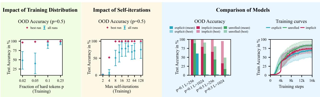
The Right panel compares the implicit approach against “unrolled” Mamba (where you just stack layers). Implicit Mamba (Red) converges much faster and more reliably than unrolled versions.
2. Large Scale Language Modeling (1.3B Parameters)
The researchers didn’t stop at toy problems. They trained Implicit Mamba2 and Implicit Llama models up to 1.3 Billion parameters on 207B tokens of the Pile dataset. This is the largest implicit model trained to date.
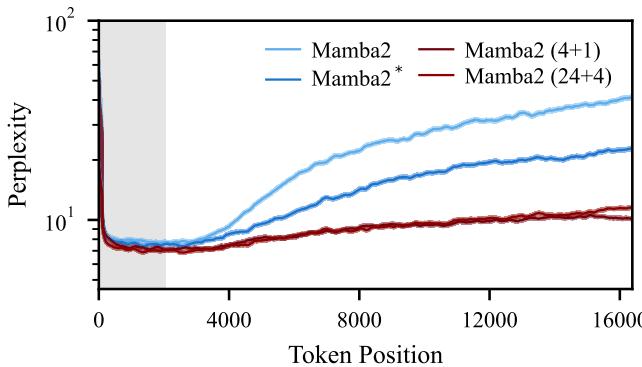
Length Extrapolation One of the most desirable features of a language model is the ability to train on short sequences and perform well on long ones. Standard models usually see their perplexity (error rate) explode when processing sequences longer than their training window.
Figure 4 below demonstrates the Length Extrapolation capabilities. The implicit models (Red and Dark Red) maintain stable, low perplexity even as the token position extends far beyond the training context (the shaded gray area). The standard Mamba2 (Light Blue) degrades significantly.
Downstream Reasoning On common sense reasoning tasks (like LAMBADA, HellaSwag, and ARC), the Implicit models generally outperformed their explicit baselines.
Interestingly, the authors also utilized the CatbAbI dataset—a benchmark for reasoning over long stories (e.g., “Where was Fred before the kitchen?”).
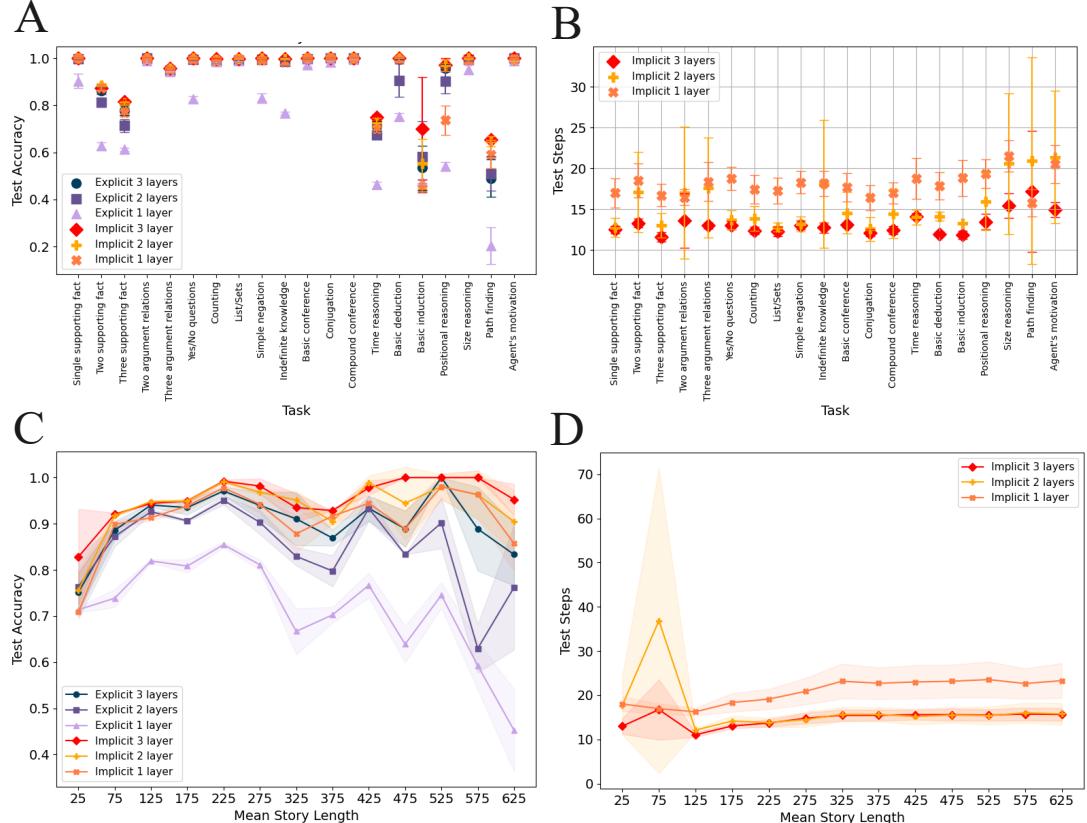
Panel (c) in Figure 13 shows that as story length increases, the accuracy of Implicit Mamba2 (Red) stays perfect, while explicit Mamba2 (Blue) collapses. Panel (d) reveals the cost: the implicit model automatically increases its number of iterations (“Test Steps”) to handle the increased difficulty. This is Adaptive Compute in action—the model thinks longer when the problem gets harder.
Conclusion & Implications
The paper Implicit Language Models are RNNs bridges a major divide in deep learning. For years, we believed we had to choose between the training efficiency of Transformers/SSMs and the state-tracking power of RNNs. This work shows that by framing the model layer as a fixed-point iteration, we can have both.
Key Takeaways:
- Implicit SSMs are RNNs: Through self-iteration, linear SSMs gain the non-linear state transitions of RNNs.
- Duality: You can train in “Simultaneous Mode” (Parallel/Fast) and run inference in “Sequential Mode” (Low Memory/RNN-like).
- Adaptive Compute: The model naturally uses more compute iterations for harder or longer sequences, solving the length generalization problem that plagues Transformers.
- Scalability: This isn’t just theory; it works at the 1.3B parameter scale with phantom gradients ensuring memory efficiency.
This approach hints at a future where Large Language Models aren’t just static predictors but dynamic systems that can “ponder” a difficult prompt until they converge on a coherent answer, all while retaining the efficiency required for massive pre-training.