Counting the Coins: How Much Randomness Do We Need for Stable Machine Learning?

In the world of machine learning and statistics, we often crave two contradictory things: consistency and privacy.

On one hand, we want reproducibility. If I run an analysis on a dataset today, and you run the same analysis on the same dataset tomorrow, we should get the same result. This is the bedrock of the scientific method.

On the other hand, we increasingly demand Differential Privacy (DP). To protect individual data points, algorithms must be randomized. If an algorithm is perfectly deterministic, it risks leaking information about the specific inputs it was trained on. Furthermore, standard training methods like Stochastic Gradient Descent (SGD) inject noise by design to improve generalization.

This creates a tension. How do we balance the need for an algorithm to be stable (producing consistent outputs) with the mathematical necessity of randomness?

A recent paper, The Role of Randomness in Stability by Max Hopkins and Shay Moran, tackles this foundational question. They treat randomness not just as “noise,” but as a computational resource—like time or memory—that can be measured. The authors ask a profound question: Exactly how many random bits—how many coin flips—do we need to achieve algorithmic stability?

In this post, we will dive deep into their findings. We will explore the connection between deterministic stability and randomized replicability, how this relates to differential privacy, and finally, how these concepts solve a major open problem in Agnostic PAC Learning.

1. The Stability Zoo: Setting the Stage

Before we measure randomness, we need to define what we mean by “stability.” The paper explores a hierarchy of stability notions, ranging from weak deterministic guarantees to strong randomized ones.

Global Stability: The Deterministic Ceiling

Imagine an algorithm \(\mathcal{A}\) that takes a dataset \(S\) and produces a model. If \(\mathcal{A}\) is deterministic, we might hope that it produces the same model even if the dataset \(S\) changes slightly (e.g., is drawn from the same underlying distribution \(D\) but has different samples).

We define Global Stability as the probability that the algorithm outputs the exact same result on two independent draws of the dataset, \(S\) and \(S'\).

Here, we are looking for the minimum collision probability over all possible data distributions \(D\).

However, there is a catch. It turns out that for any non-trivial statistical task, it is impossible for a deterministic algorithm to be perfectly globally stable. In fact, the “Global Stability” parameter is universally capped at \(1/2\).

Why is it capped? Intuitively, imagine a classification problem where the data distribution shifts from “mostly Class A” to “mostly Class B.” At some point in that transition, the optimal model must switch from predicting A to predicting B. At that exact tipping point, a deterministic algorithm must effectively “choose a side.” If it chooses A, it’s wrong for B, and vice versa. This inevitable flip creates instability.

This leads us to the “Heavy Hitter” definition. We say an algorithm is \(\eta\)-globally stable if, for every distribution, there exists a specific output (a “heavy hitter”) that appears with probability at least \(\eta\).

Replicability: Adding Shared Randomness

Since deterministic algorithms are capped at a stability of \(1/2\), how do we achieve the scientific ideal of near-certain reproducibility? The answer lies in Replicability.

Replicability allows the algorithm to use internal randomness, but with a twist: the randomness is shared across runs. Think of this as a “seed” for a random number generator that is published alongside the algorithm.

An algorithm is \(\rho\)-replicable if, given two independent datasets \(S\) and \(S'\) and a shared random string \(r\), the outputs are identical with high probability:

This is a much stronger guarantee. It allows us to bypass the \(1/2\) barrier. But it comes at a cost: we need to generate and share that random string \(r\). This brings us to the core metric of the paper: Certificate Complexity.

Certificate Complexity (\(C_{Rep}\)) is simply the minimum number of random bits (the length of \(r\)) required to achieve high replicability (specifically, better than \(1/2\)).

Differential Privacy (DP)

Finally, we have Differential Privacy. An algorithm is \((\varepsilon, \delta)\)-DP if its output distribution doesn’t change much when we change a single data point in the input \(S\).

Like replicability, DP inherently requires randomness. The paper introduces DP Complexity, which counts the random bits needed to satisfy this privacy definition while solving a task.

2. The Core Insight: A Weak-to-Strong Boosting Theorem

The heart of Hopkins and Moran’s work is a surprising equivalence between the “weak” notion of Global Stability (which requires no randomness but has low probability) and the “strong” notion of Replicability (which has high probability but requires randomness).

They prove a “Weak-to-Strong” Boosting Theorem. The theorem states that the number of random bits you need to make an algorithm replicable is effectively determined by the best stability you could achieve deterministically.

The Equivalence

The authors derive a tight bound relating Global Stability complexity (\(C_{Glob}\)) and Certificate Complexity (\(C_{Rep}\)).

This equation is profound. It says that Global Stability and Certificate Complexity are essentially the same resource. If you have a deterministic algorithm that hits the right answer with probability \(\eta\), you can boost it to be fully replicable using roughly \(\log(1/\eta)\) random bits.

How the Boosting Works (The Thresholding Trick)

How do you magically turn a “weak” heavy hitter (an output that appears, say, 10% of the time) into a “strong” replicable output (one that appears 99% of the time using shared randomness)?

The authors employ a technique involving discretized rounding or random thresholds.

Step 1: Estimate Probabilities First, run the weak global algorithm many times on fresh data to estimate the empirical probability mass of every possible output hypothesis. Let’s say hypothesis \(y_1\) appears 12% of the time, \(y_2\) appears 8% of the time, and so on.

Step 2: The Random Threshold We need to pick one hypothesis consistently. We can’t just pick the max because if two hypotheses have similar probabilities (e.g., 12% vs 12.1%), small sampling noise will make the max flip-flop between them, breaking replicability.

Instead, we use shared randomness to pick a random threshold \(t\).

Step 3: Selection We select the first hypothesis whose empirical probability exceeds the threshold \(t\).

Why does this work? The only time this method fails is if the true probability of a hypothesis is very close to the random threshold \(t\). In that case, sampling noise might push the empirical estimate above or below \(t\) in different runs.

But here is the clever part: because the threshold \(t\) is chosen randomly, the probability that it lands in a “danger zone” (right next to a hypothesis’s true probability) is low.

The authors illustrate this with a “Thresholding Procedure.”

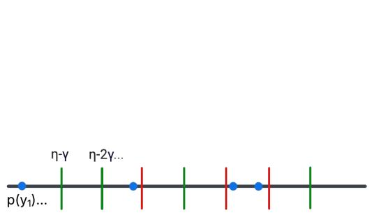
In the figure above:

• The Blue dots represent the probabilities of the “heavy hitter” hypotheses.
• The Vertical lines represent possible random thresholds (determined by the random bits).
• The Green lines are “safe” thresholds—they are far enough away from any blue dot that noise won’t cause a flip.
• The Red lines would be “unsafe” thresholds.

By using just a few bits of randomness to select a green threshold, we ensure that both runs of the algorithm (on \(S\) and \(S'\)) will agree on which hypothesis crosses the line.

This technique proves that you can “buy” stability. The cost is exactly \(\log(1/\eta)\) bits, where \(\eta\) is the frequency of your heavy hitter.

3. Connecting Stability to Privacy

Having established that Replicability and Global Stability are two sides of the same coin, the authors turn to Differential Privacy (DP).

DP is usually more complex because it depends on sample size \(n\) and confidence \(\beta\). The authors define User-Level DP, where we protect an entire user’s dataset rather than a single row. This simplifies the math and strengthens the connection.

Stability \(\to\) DP

The authors show that if you have a Globally Stable algorithm, you can make it Differentially Private with very little extra randomness.

The transformation involves three steps:

1. Heavy Hitters: Use the globally stable algorithm to find a list of likely outputs.
2. DP Selection: Use a standard privacy mechanism (like the Exponential Mechanism) to select one hypothesis from that list.
3. Bounded Support: Crucially, ensure the algorithm always outputs something from a small, fixed set (the support).

The authors prove that any distribution with small support can be approximated using very few random bits. This allows them to construct a DP algorithm that is extremely efficient in terms of randomness.

DP \(\to\) Stability

Does the reverse hold? If an algorithm is Differentially Private, does it imply it is Globally Stable?

Yes. The paper leverages a concept called Perfect Generalization. It turns out that any sufficiently private algorithm is also “perfectly generalizing,” meaning its output distribution on a specific dataset looks very similar to its output distribution on the general population.

If the output distribution is stable, it must have “heavy hitters” (outputs that appear frequently). As we learned in Section 2, if you have heavy hitters, you have Global Stability.

Therefore, the circle is complete:

1. Global Stability \(\approx\) Replicability (via Boosting)
2. Global Stability \(\leftrightarrow\) Differential Privacy (via Heavy Hitters and DP Selection)

4. Solving the Agnostic PAC Learning Problem

The theoretical machinery above isn’t just for show. The authors apply it to a concrete open problem in learning theory: Agnostic PAC Learning.

The Setup

• PAC Learning: “Probably Approximately Correct” learning. We want an algorithm that, with high probability, outputs a classifier with low error.
• Agnostic: We don’t assume the data perfectly fits our model class (e.g., we are trying to fit a line to data that isn’t perfectly linear). We just want the best possible fit.
• The Question: How much randomness is needed to learn a hypothesis class \(H\) in the agnostic setting?

Previous work established that in the “Realizable” setting (where a perfect model exists), the randomness complexity is controlled by the Littlestone Dimension (\(d\)). However, it was unknown if this held for the harder Agnostic setting.

The Result

The authors prove that Agnostic PAC Learning is possible with bounded randomness if and only if the Littlestone Dimension is finite.

Specifically, they provide a learner with Certificate Complexity (random bits) that scales with the dimension \(d\) and logarithmically with the error \(\alpha\).

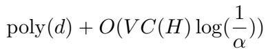
Here, \(VC(H)\) is the VC-dimension (a measure of complexity usually smaller than Littlestone dimension). The term \(O(\log(1/\alpha))\) is the crucial win—it shows the randomness cost grows very slowly as we demand higher accuracy.

The Algorithm: Reduce, Boost, Prune

How do they achieve this? They combine their new “Stability Boosting” theorem with a reduction technique.

1. Realizable List-Stable Learner: They start with an existing algorithm for the easier (realizable) case. This algorithm outputs a list of candidate hypotheses.
2. Agnostic Reduction: They run this realizable learner on many unlabeled samples to generate a massive pool of potential hypotheses.
3. Pruning: This pool is too big. They use a fresh labeled dataset to test these hypotheses and “prune” the ones with high error.
4. Heavy Hitter: They argue that the optimal hypothesis will appear frequently in this pruned list.
5. Randomness Injection: Finally, they apply the Stability Boosting (thresholding) trick to pick one specific hypothesis from this list using shared randomness.

This chain of logic converts a messy, agnostic learning problem into a clean, replicable algorithm using a precise amount of randomness.

5. Conclusion and Implications

The paper The Role of Randomness in Stability offers a unifying perspective on algorithmic stability.

For students and practitioners, the key takeaways are:

1. Randomness is a Resource: We can quantify exactly how many bits of randomness are needed for stability. It’s not infinite; it’s often just logarithmic in the difficulty of the problem.
2. Equivalence: Deterministic stability (finding a heavy hitter) and Randomized Replicability (agreeing on an output) are computationally equivalent. You can trade a small amount of randomness to upgrade the former to the latter.
3. Privacy Connection: Differential Privacy is intimately linked to these concepts. If you can solve a problem privately, you can solve it stably, and vice versa.
4. Learning Theory: This framework resolves the randomness complexity of Agnostic Learning, proving that efficient, stable learning is possible even when the data is noisy.

This work helps demystify the “black box” of randomness in machine learning. It tells us that while we cannot eliminate the need for coin flips in privacy and stability, we can count them, optimize them, and understand exactly what we are buying with each bit.