Tightening the belt - Improving Sparse Variational GPs with New Bounds

Gaussian Processes (GPs) are the Swiss Army knife of probabilistic modeling. They offer flexibility, non-parametric curve fitting, and, perhaps most importantly, principled uncertainty quantification. However, they have a well-known Achilles’ heel: scalability. The computational cost of a standard GP grows cubically with the number of data points (\(O(N^3)\)), making them impractical for datasets larger than a few thousand points.

For over a decade, the standard solution to this problem has been the Sparse Variational Gaussian Process (SVGP). Introduced notably by Titsias in 2009, this method uses “inducing points” and variational inference to reduce the complexity to \(O(NM^2)\), where \(M\) is a small number of inducing points. It has become the default setting in major GP libraries like GPflow and GPyTorch.

But here is the catch: to make the math tractable, the standard SVGP makes a fundamental assumption about the relationship between the inducing points and the training data. For years, this assumption was viewed as necessary. A new research paper, “New Bounds for Sparse Variational Gaussian Processes,” challenges this status quo. The authors demonstrate that we can relax this assumption, derived a strictly tighter Evidence Lower Bound (ELBO), and achieve better predictive performance—all without increasing the computational complexity class.

In this post, we will tear down the SVGP derivation, identify the exact moment the approximation can be improved, and walk through the derivation of this new, tighter bound.

Background: The Standard SVGP Recipe

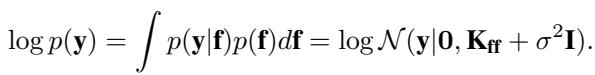
To understand the innovation, we first need to establish the baseline. A Gaussian Process places a distribution over functions \(f\). Given input data \(\mathbf{X}\), the function values \(\mathbf{f}\) follow a multivariate normal distribution defined by a kernel function \(k\):

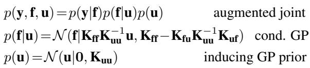
In a regression setting, we observe noisy targets \(\mathbf{y}\). The joint probability of our targets and the latent function values is:

Learning the hyperparameters (like lengthscales and signal variance) involves maximizing the log marginal likelihood, \(\log p(\mathbf{y})\). However, calculating this requires inverting the covariance matrix \(\mathbf{K}_{ff} + \sigma^2 \mathbf{I}\), which is the source of the dreaded \(O(N^3)\) bottleneck.

The Variational Approach

To scale this up, SVGP introduces inducing variables \(\mathbf{u}\). These are function values at a set of \(M\) locations \(\mathbf{Z}\), distinct from the training data \(\mathbf{X}\). The core idea is that these \(M\) points can summarize the function well enough to predict the remaining \(N\) points.

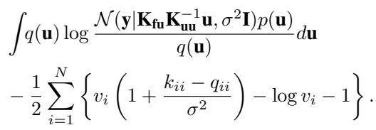
We augment the model with these inducing variables. A crucial part of the SVGP framework is how we define the joint distribution of the data \(\mathbf{f}\) and the inducing variables \(\mathbf{u}\). We write the joint prior as \(p(\mathbf{f}, \mathbf{u}) = p(\mathbf{f}|\mathbf{u})p(\mathbf{u})\), where \(p(\mathbf{f}|\mathbf{u})\) is the conditional Gaussian distribution.

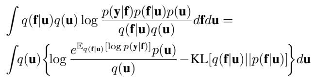
In Variational Inference, we approximate the true posterior \(p(\mathbf{f}, \mathbf{u} | \mathbf{y})\) with a simpler distribution \(q(\mathbf{f}, \mathbf{u})\). We then minimize the Kullback-Leibler (KL) divergence between \(q\) and the true posterior, which is equivalent to maximizing the Evidence Lower Bound (ELBO).

The Standard Assumption: In the original SVGP method (Titsias, 2009), the variational posterior is factorized in a very specific way:

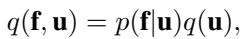
Here, \(q(\mathbf{u})\) is a free variational distribution (usually Gaussian) that we optimize. However, \(p(\mathbf{f}|\mathbf{u})\) is the exact conditional prior.

This choice is convenient because it causes terms to cancel out nicely during the derivation, leading to a computationally efficient bound. The resulting “collapsed” bound (where \(q(\mathbf{u})\) is optimally solved for) looks like this:

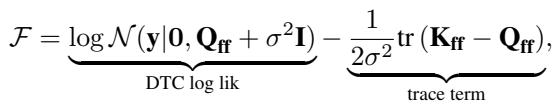
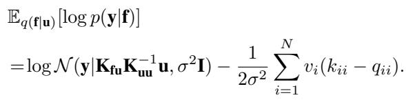
This formula is likely familiar to anyone who has implemented SVGP. The first term is a data fit term (using the Nyström approximation \(\mathbf{Q}_{ff}\)), and the second term is a regularization trace term.

The Limitation

The restriction \(q(\mathbf{f}, \mathbf{u}) = p(\mathbf{f}|\mathbf{u})q(\mathbf{u})\) implies that given the inducing points \(\mathbf{u}\), the training points \(\mathbf{f}\) behave exactly according to the prior. Information from the observed data \(\mathbf{y}\) only flows into \(\mathbf{f}\) through \(\mathbf{u}\).

But is this optimal? If we knew the true posterior \(p(\mathbf{f}|\mathbf{u}, \mathbf{y})\), would it look like the prior \(p(\mathbf{f}|\mathbf{u})\)? generally, no. The true posterior would incorporate information from \(\mathbf{y}\) to adjust the correlations between \(\mathbf{f}\) and \(\mathbf{u}\). By forcing our approximation to use the prior conditional, we are limiting the expressiveness of our model, leading to a looser bound and potentially biased hyperparameter learning (often manifesting as over-estimated observation noise).

The Core Method: Relaxing the Conditional

The researchers propose a method to tighten the bound by replacing the fixed prior \(p(\mathbf{f}|\mathbf{u})\) with a parameterized distribution \(q(\mathbf{f}|\mathbf{u})\).

1. Analyzing the Exact Posterior

To design a better approximation, let’s look at what the exact conditional posterior \(p(\mathbf{f}|\mathbf{u}, \mathbf{y})\) actually looks like. If we could use this exact distribution, the KL divergence would vanish, and our approximation would be perfect.

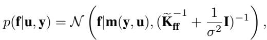
In this equation, \(\widetilde{\mathbf{K}}_{ff} = \mathbf{K}_{ff} - \mathbf{Q}_{ff}\). The mean \(\mathbf{m}(\mathbf{y}, \mathbf{u})\) is complex, but the covariance structure is key. The precision matrix (inverse covariance) is \((\widetilde{\mathbf{K}}_{ff}^{-1} + \frac{1}{\sigma^2}\mathbf{I})\).

We can rewrite the covariance of this exact posterior using matrix identities:

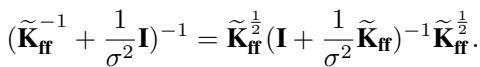
This structure gives us a hint. The exact posterior covariance is “smaller” (more precise) than the prior covariance because of the data term \(\frac{1}{\sigma^2}\). The standard SVGP effectively ignores this reduction in variance for the conditional part.

2. The New Variational Family

The paper proposes a new form for \(q(\mathbf{f}|\mathbf{u})\) that mimics the structure of the exact posterior but remains computationally tractable. Specifically, they introduce a diagonal matrix of variational parameters \(\mathbf{V} = \text{diag}(v_1, \dots, v_N)\).

The proposed distribution is:

Here is the logic behind this choice:

1. Mean: It keeps the same mean as the prior, \(\mathbf{K}_{fu}\mathbf{K}_{uu}^{-1}\mathbf{u}\). This keeps the expectations tractable.
2. Covariance: It replaces the inverse term \((\mathbf{I} + \dots)^{-1}\) from the exact posterior with the diagonal matrix \(\mathbf{V}\).

This introduces \(N\) new parameters (\(v_1\) to \(v_N\)). If \(V = I\) (identity matrix), we recover the standard SVGP. If optimizing \(V\) allows us to lower the variance, we get a tighter bound.

3. Deriving the New Bound

With this new \(q(\mathbf{f}|\mathbf{u})\), the ELBO derivation changes. We now have to compute the KL divergence between our new \(q(\mathbf{f}|\mathbf{u})\) and the prior \(p(\mathbf{f}|\mathbf{u})\).

The derivation involves two main components:

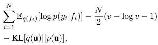
1. The KL Term: Since both distributions are Gaussian and share the same mean, the KL divergence simplifies significantly. It depends only on the trace and determinant of the diagonal matrix \(\mathbf{V}\). \[ \text{KL} = \frac{1}{2}\sum_{i=1}^N (v_i - \log v_i - 1) \]
2. The Expected Log Likelihood: This term is modified by the new covariance structure.

Combining these, we get an objective function that depends on \(\mathbf{u}\), the hyperparameters, and our new parameters \(v_i\).

4. The “Collapsed” Tighter Bound

Here is the elegant part. We don’t actually need to use gradient descent to find \(v_i\). The bound above is concave with respect to \(v_i\). We can take the derivative, set it to zero, and find the optimal \(v_i^*\) analytically:

When we substitute this optimal \(v_i^*\) back into the bound (and also solve for the optimal \(q(\mathbf{u})\) as in standard SVGP), we arrive at the new collapsed bound:

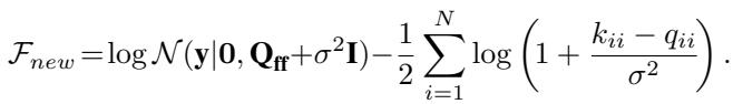
Let’s compare this to the old bound:

• Old Trace Term: \(-\frac{1}{2\sigma^2} \sum (k_{ii} - q_{ii})\)
• New Log Term: \(-\frac{1}{2} \sum \log(1 + \frac{k_{ii} - q_{ii}}{\sigma^2})\)

Using the inequality \(\log(1+x) \le x\), we can mathematically prove that the new term is always greater than or equal to the old term. Since we are maximizing a lower bound, the new bound is strictly tighter (better) whenever the inducing points do not perfectly explain the data (i.e., when \(k_{ii} - q_{ii} > 0\)).

Essentially, the new method replaces a linear penalty on the approximation error with a logarithmic one, which is more forgiving and mathematically closer to the true marginal likelihood.

Efficient Training

One of the strengths of SVGP is its ability to train using stochastic gradient descent (minibatches), enabling it to scale to millions of data points. Does this new method break that?

No. The uncollapsed bound (where we keep \(q(\mathbf{u})\) as a variational parameter to be optimized) also benefits from the analytic solution for \(v_i\).

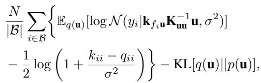
This equation looks complicated, but it is structurally identical to the standard stochastic ELBO used in software like GPflow, with just the scalar regularization term changed.

• Complexity: The complexity remains dominated by the matrix operations on the inducing points, \(O(M^3)\) or \(O(NM^2)\), depending on the implementation.
• Storage: We do not need to store the \(N\) parameters \(v_i\); they are computed on the fly from the current kernel hyperparameters and inducing points.

Extension: Non-Gaussian Likelihoods

What if we are doing classification or modeling counts (Poisson regression)? In these cases, the likelihood \(p(y|f)\) is not Gaussian, and we cannot easily integrate out everything.

The standard approach uses quadrature or Monte Carlo sampling for the expected log-likelihood. The new method can still be applied, but optimizing a distinct \(v_i\) for every data point becomes expensive because the optimal \(v_i\) no longer has a closed-form solution.

The authors propose a compromise: use a spherical \(\mathbf{V} = v\mathbf{I}\). We learn a single scalar \(v\) that adjusts the variance for all data points.

This introduces just one extra parameter (\(v\)) to the optimization, maintaining efficiency while still offering a tighter bound than the standard formulation (which effectively forces \(v=1\)).

Experiments and Results

The paper validates the new bound on several datasets.

1. Snelson 1D Regression (The Visual Proof)

The Snelson dataset is a classic “Hello World” for GPs. It has a complex function with varying density of data.

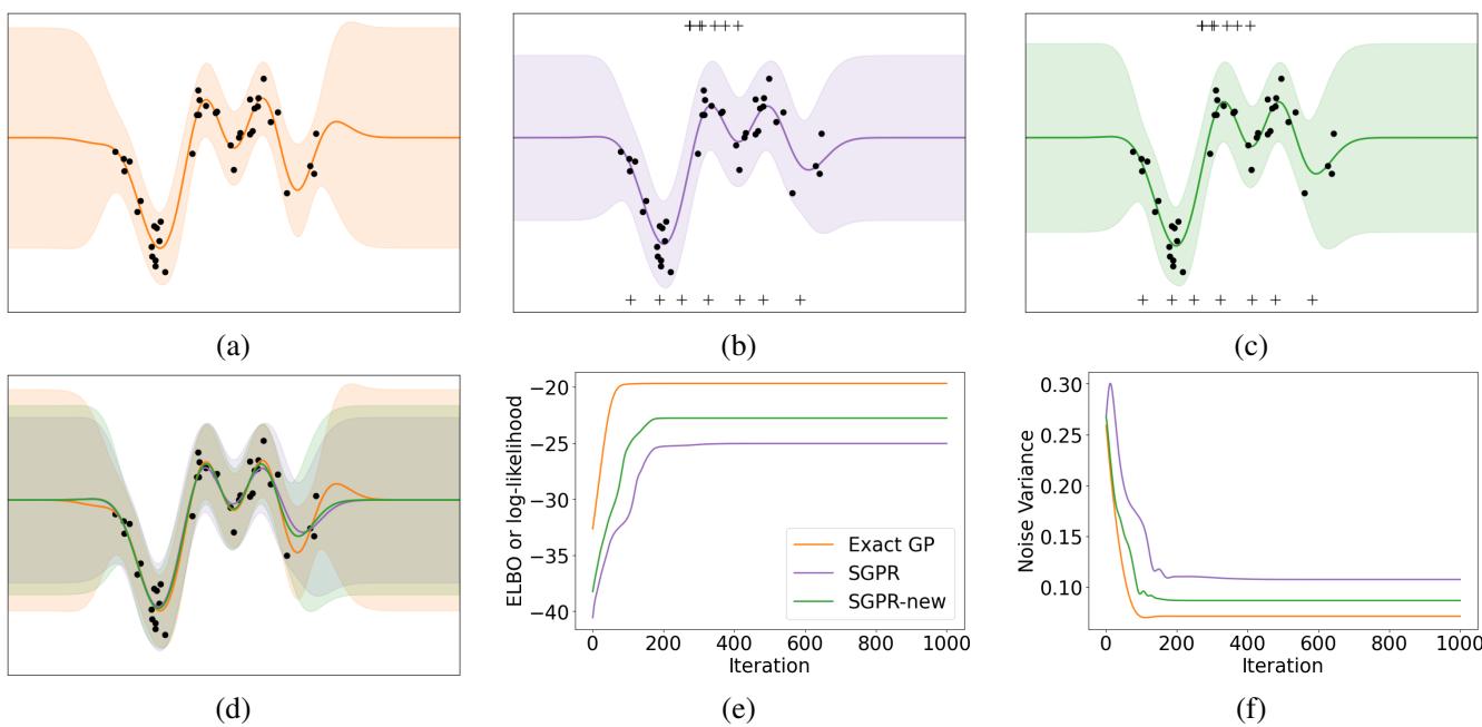
• Figure (a): The Exact GP (ground truth).
• Figure (b): Standard SGPR (old bound). Notice the predictive variance is somewhat inflated.
• Figure (c): SGPR-new (proposed). The variance is tighter and matches the exact GP much more closely.
• Figure (f): This plot shows the learned noise variance \(\sigma^2\) during training. The standard SGPR (purple) converges to a higher noise value to compensate for its looser bound. The new method (green) converges to a lower noise value, almost identical to the exact GP (orange).

This confirms the hypothesis: the new bound reduces the “underfitting” bias where SVGP tends to overestimate observation noise.

2. Medium Scale Benchmarks

The authors compared the methods on UCI regression datasets (Pol, Bike, Elevators).

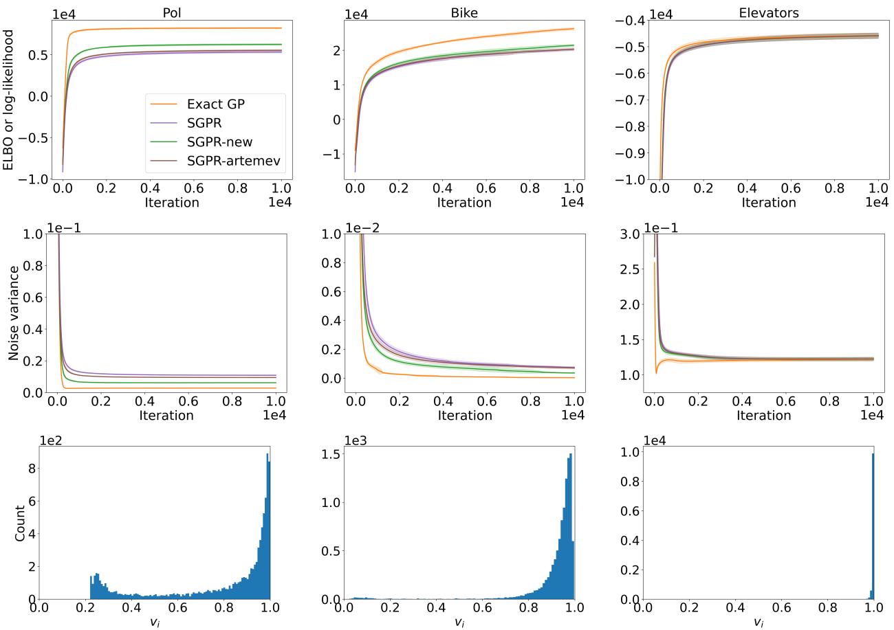
In Figure 2, we see the optimization traces.

• Top Row (ELBO): The Green line (SGPR-new) consistently achieves a higher ELBO than the standard method.
• Bottom Row (Histograms): This shows the distribution of the optimal \(v_i\) values. If the standard SVGP were optimal, all \(v_i\) would be 1.0. The fact that they cluster around 0.8-0.9 indicates that the standard approximation was indeed too loose, and the new parameters are actively correcting the covariance.

The table of results reinforces this:

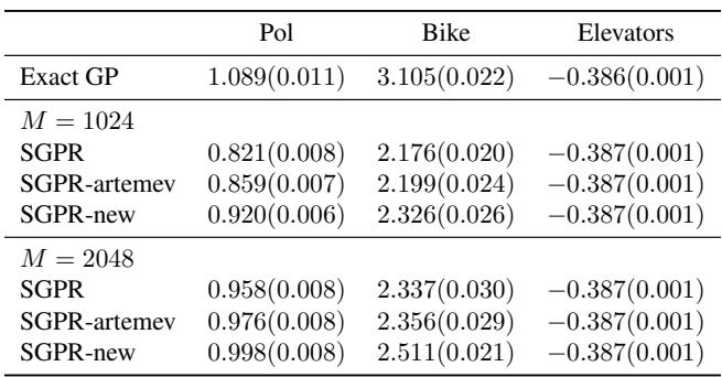
The proposed method (SGPR-new) achieves higher test log-likelihoods, indicating better generalization.

3. Large Scale & Poisson Regression

For large datasets (millions of points) where exact GPs are impossible, the stochastic version of the new bound was compared against the standard SVGP.

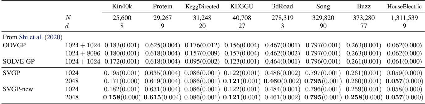
Across datasets like “HouseElectric” (1.3 million points), the new method consistently edges out the standard SVGP and other baselines.

Finally, for Poisson regression (Count data), they used the scalar \(v\) approximation.

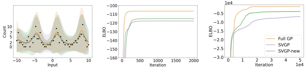
The Left panel shows the fit on count data. The Green line (New) tracks the Orange line (Full GP) better than the Purple line (Standard SVGP). The ELBO plots (Middle/Right) show a clear gap, proving that even a single scalar parameter \(v\) can significantly improve the approximation quality for non-conjugate likelihoods.

Conclusion

The contribution of this paper is a rigorous “free lunch” for the Gaussian Process community. By relaxing the rigid assumption that \(q(\mathbf{f}|\mathbf{u}) = p(\mathbf{f}|\mathbf{u})\), the authors derived a new bound that is:

1. Strictly Tighter: Mathematically proven to be a better lower bound on the model evidence.
2. Same Complexity: It fits into the same \(O(NM^2)\) computational class.
3. Easy to Implement: It requires changing a single term in the loss function (trace term \(\to\) log term) for the regression case.

For students and practitioners, this result highlights the importance of questioning “standard” assumptions in variational inference. A small change in the variational family can lead to significant gains in model accuracy and hyperparameter learning, without requiring more expensive hardware. As GP software libraries adopt these bounds, we can expect sparse GPs to become slightly more accurate and robust by default.