Introduction

In the rapidly evolving world of generative AI, we are often forced to choose between speed, quality, and training stability. For years, Generative Adversarial Networks (GANs) offered lightning-fast, one-step generation but suffered from notoriously unstable training dynamics (the famous “mode collapse”). Then came Diffusion Models, which revolutionized the field with stable training and incredible image quality, but at a significant cost: sampling is slow, requiring dozens or hundreds of iterative steps to denoise a single image.

The Holy Grail of generative modeling is to combine the best of both worlds: the one-step speed of GANs with the training stability and quality of Diffusion Models.

Researchers from MIT have proposed a novel framework that might just be the answer. It is called Score-of-Mixture Training (SMT). This method allows for training high-quality one-step generative models from scratch without the instability of adversarial training or the complexity of simulating probability flow ODEs used in consistency models.

In this deep dive, we will explore how SMT works, the mathematical intuition behind it, and how it uses a clever “mixture” concept to stabilize the learning process.

The Generative Landscape

To understand why SMT is significant, we first need to look at where it sits in the current landscape of generative models.

1. GANs: Train a generator to fool a discriminator. They minimize the Jensen–Shannon divergence (JSD). While fast (one-step), the adversarial min-max game is difficult to stabilize.
2. Diffusion Models: Learn to reverse a noise process. They use Denoising Score Matching (DSM) to learn the “score” (the gradient of the data distribution). Training is very stable, but generation is slow.
3. Consistency Models: Try to distill the slow diffusion process into a single step by mapping points on a trajectory to their origin. While promising, training them from scratch can be finicky regarding noise schedules.

The authors of SMT propose a fourth path. They aim to minimize a statistical divergence directly using score matching, removing the need for a discriminator (like GANs) or iterative integration (like Diffusion).

As shown in Table 1, SMT (and its distillation variant, SMD) occupies a unique spot: it offers stable, one-step generation without requiring a pretrained model (though it can use one if available).

The Core Intuition: Score of Mixtures

The central innovation of this paper is shifting the focus from standard divergences to a family of divergences called the \(\alpha\)-skew Jensen–Shannon Divergence (\(\alpha\)-JSD).

The Mathematics of \(\alpha\)-JSD

Standard diffusion distillation often minimizes the Reverse KL Divergence. GANs minimize the standard JSD. The \(\alpha\)-JSD is a generalized family that interpolates between these.

Here is the intuition:

• When \(\alpha \to 0\), it behaves like the Forward KL Divergence (mode-covering).
• When \(\alpha \to 1\), it behaves like the Reverse KL Divergence (mode-seeking).
• When \(\alpha = 0.5\), it is the standard JSD used in GANs.

By minimizing this divergence across a range of \(\alpha\) values, the model can learn both to cover the diversity of the data and to generate sharp, high-quality modes.

The Gradient and the “Score”

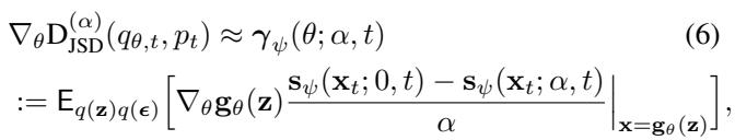
To train a neural network generator, we need to calculate the gradient of this divergence with respect to the generator’s parameters (\(\theta\)). The researchers derived a fascinating relationship: the gradient of the \(\alpha\)-JSD depends on the score of the mixture distribution.

The “score” function, \(\mathbf{s}(\mathbf{x})\), is simply the gradient of the log-probability density with respect to the data: \(\nabla_\mathbf{x} \log p(\mathbf{x})\). It points in the direction where data is more likely to exist.

The gradient for the generator update looks like this:

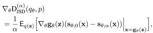
Notice the term \((\mathbf{s}_{\theta;0}(\mathbf{x}) - \mathbf{s}_{\theta;\alpha}(\mathbf{x}))\).

• \(\mathbf{s}_{\theta;0}(\mathbf{x})\) is essentially the score of the generated (fake) distribution.
• \(\mathbf{s}_{\theta;\alpha}(\mathbf{x})\) is the score of the mixture distribution: \(\alpha p(\mathbf{x}) + (1-\alpha)q_\theta(\mathbf{x})\).

This tells us that to update the generator, we don’t need a discriminator to say “yes/no.” Instead, we need a model that can estimate the score of a mix of real and fake data.

Score-of-Mixture Training (SMT): Training from Scratch

The SMT framework creates a stable training loop by alternating between two tasks:

1. Score Estimation: Train a network to estimate the score of the mixture of real and fake distributions.
2. Generator Update: Use those estimated scores to push the generator’s output toward the real data distribution.

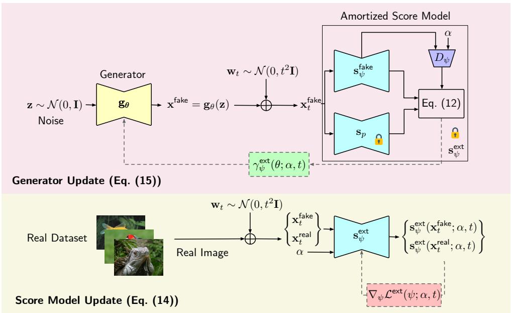
The Architecture

To make this efficient, the authors introduce an Amortized Score Model. Instead of training separate models for every possible mixture weight \(\alpha\), they train a single neural network \(\mathbf{s}_\psi(\mathbf{x}; \alpha, t)\) that takes \(\alpha\) and the noise level \(t\) as inputs.

This creates a highly efficient system. The score model learns the geometry of how real and fake distributions overlap across different noise levels.

The Training Loop

Let’s visualize the entire process.

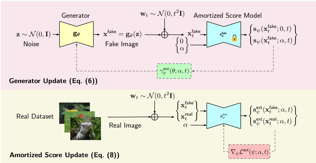
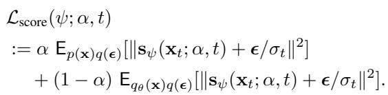
In the Bottom path (Score Update): We take real images and fake images (generated by the current model). We mix them implicitly by asking the score model to learn the score of the mixture distribution. This is done using standard Denoising Score Matching (DSM), which is known to be very stable. The loss function looks like this:

In the Top path (Generator Update): We freeze the score model. We generate fake images, add noise, and then calculate the gradient based on the difference between the “pure” fake score and the “mixture” score. This gradient nudges the generator’s parameters \(\theta\) so that the generated distribution moves closer to the real distribution.

The generator update uses an approximation derived from the \(\alpha\)-JSD gradient:

This approach avoids the “min-max” instability of GANs because the score model is always trying to minimize a regression loss (how well it predicts noise), which is a much easier optimization task than trying to beat a generator in a zero-sum game.

Adaptive Weighting

One implementation detail that significantly boosts performance is how the gradients are weighted. The authors introduce a specific weighting term \(w(\mathbf{x}_t, \mathbf{x}, \alpha, t)\) to ensure the training signal remains strong and stable throughout the process.

This weighting combines standard diffusion weights with a term specific to the geometry of the mixture, ensuring that neither the \(\alpha \to 0\) nor \(\alpha \to 1\) extremes dominate the learning unproductively.

Score-of-Mixture Distillation (SMD)

What if you already have a powerful, pretrained diffusion model (like Stable Diffusion or an ImageNet model)? You don’t want to learn everything from scratch. You just want to distill that slow model into a fast one-step generator.

This is where Score-of-Mixture Distillation (SMD) comes in.

In SMD, we treat the pretrained model as the “ground truth” score for the real data, \(\mathbf{s}_p(\mathbf{x})\). Because we have this explicit representation of the real data, we don’t need to learn the mixture score “blindly.” We can decompose the mixture score explicitly:

Here, \(D_{\theta;\alpha}\) acts somewhat like a discriminator—it represents the probability ratio between real and fake data.

In the SMD framework:

1. We learn a fake score model \(\mathbf{s}_{\psi}^{\text{fake}}\) (the score of the current generator’s distribution).
2. We learn a discriminator \(D_\psi\) (the density ratio).
3. We combine them using the pretrained teacher \(\mathbf{s}_p\) to get the mixture score.

This explicit parameterization allows for very efficient distillation. The generator minimizes the \(\alpha\)-JSD using the pretrained model as a guide, achieving state-of-the-art results with a fraction of the compute required by other methods.

Experiments and Results

The authors tested SMT and SMD on two standard benchmarks: ImageNet 64x64 and CIFAR-10. The metric used is FID (Fréchet Inception Distance), where lower is better.

Quantitative Performance

The results are highly impressive. As shown in Table 2, SMT (Training from scratch) achieves an FID of 3.23 on ImageNet 64x64. This outperforms Consistency Training (CT) and is competitive with “iCT-deep,” a model with double the parameters.

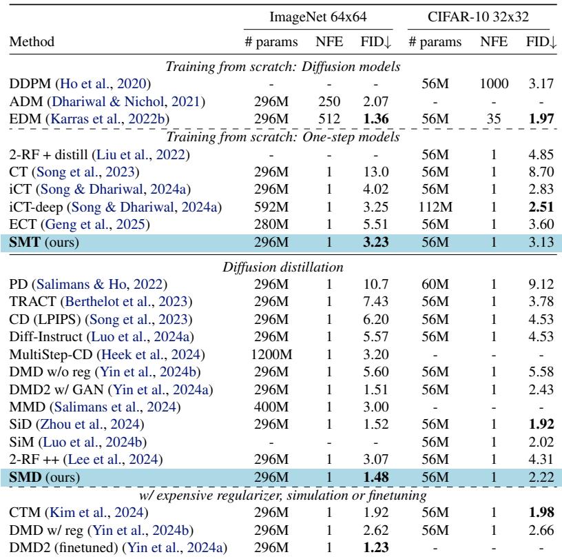
For Distillation (SMD), the results are even stronger. SMD achieves an FID of 1.48 on ImageNet 64x64. This beats or rivals complicated methods like Consistency Trajectory Models (CTM) and Diffusion Matching Distillation (DMD2) while being simpler to implement.

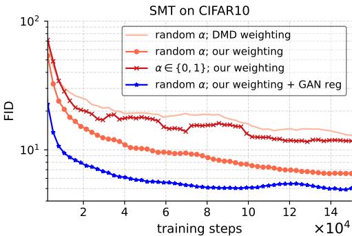
Training Stability

One of the main claims of the paper is stability. In GANs, loss curves often oscillate wildly. In Consistency Models, tuning the noise schedule is delicate.

The authors visualized the training dynamics of SMT.

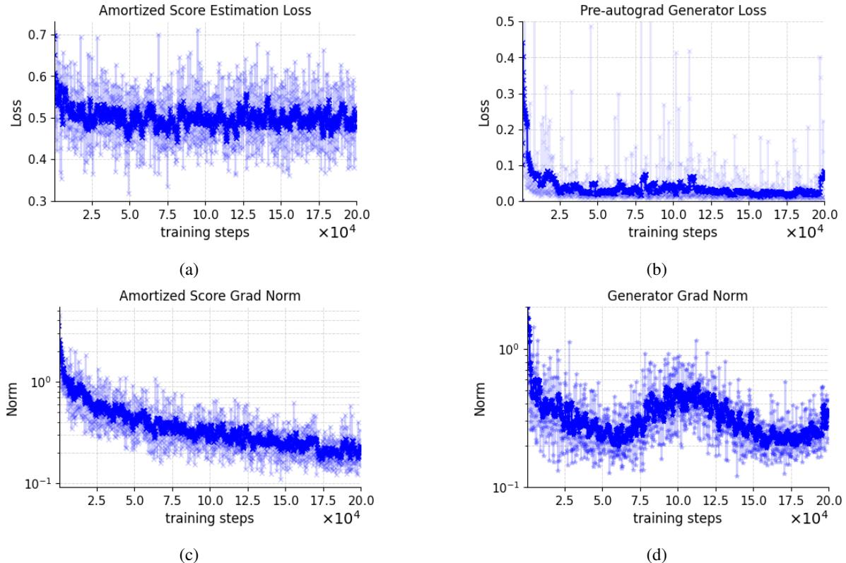
The curves in Figure 8 show a smooth, steady convergence. The loss does not explode, and the gradient norms remain healthy. This confirms that estimating the score of mixtures via DSM provides a robust signal for the generator.

Furthermore, looking at the FID evolution during training shows that the method consistently improves sample quality over time without the erratic behavior often seen in adversarial training.

Visual Quality

The numbers are good, but what do the images look like?

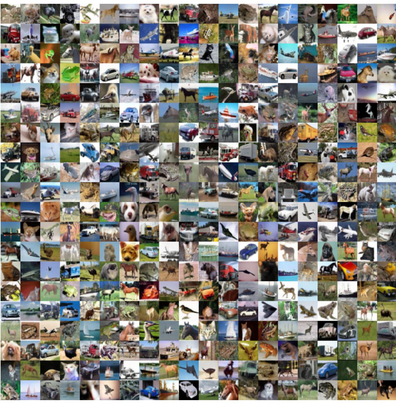
Here are samples from the SMT model (trained from scratch) on ImageNet. The diversity and fidelity are remarkable for a one-step model that doesn’t rely on a pretrained backbone.

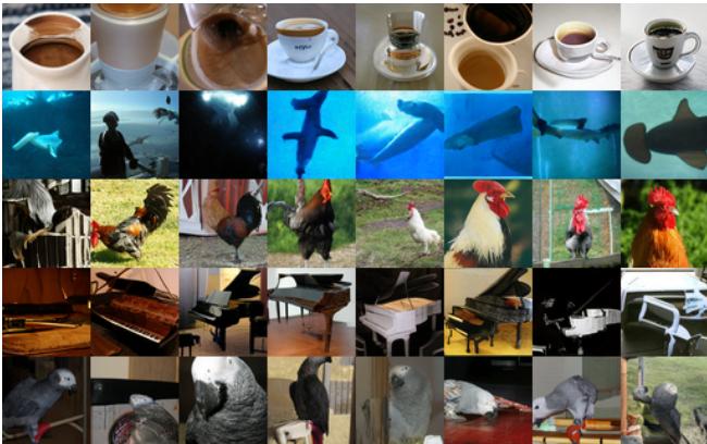
And here are samples from the SMD model (distillation) on CIFAR-10. The images are sharp and indistinguishable from the training data.

Latent Space Interpolation

A good generative model shouldn’t just memorize training data; it should learn a meaningful latent space. The authors demonstrated this by interpolating between random noise vectors.

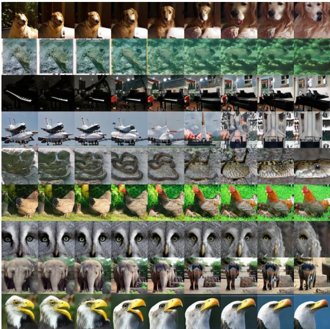
In Figure 6, you can see smooth transitions between different images (e.g., the dog in the top row changing pose). This indicates the generator has learned a structured and continuous representation of the data manifold.

Conclusion

The “Score-of-Mixture” framework represents a significant step forward in generative modeling. It successfully decouples the generation of high-quality samples from the computational burden of iterative diffusion processes, without succumbing to the instability of GANs.

Key Takeaways:

• Simplicity: SMT minimizes a statistical divergence (\(\alpha\)-JSD) directly using score estimation.
• Stability: By leveraging Denoising Score Matching, it avoids the pitfalls of adversarial min-max optimization.
• Flexibility: It works both for training from scratch (SMT) and for distilling heavy pretrained models (SMD).
• Performance: It achieves state-of-the-art or competitive one-step generation results on standard benchmarks.

For students and researchers, this paper provides a bridge between the geometric insights of information theory (divergences) and the practical power of modern score-based deep learning. It suggests that the future of fast generation might not require new architectures, but rather a better understanding of how we compare and mix probability distributions.