In the world of machine learning theory, there is often a stark difference between what works for two classes and what works for three or more. We see this in various domains, but a recent paper titled “Statistical Query Hardness of Multiclass Linear Classification with Random Classification Noise” highlights a particularly dramatic gap in the complexity of learning from noisy data.

The problem of Multiclass Linear Classification (MLC) is a textbook staple: given data points in a high-dimensional space, can we find linear boundaries that separate them into \(k\) distinct classes? When the labels are clean (perfectly accurate), this is solvable efficiently. When we have Random Classification Noise (RCN)—where labels are randomly flipped based on a noise matrix—the story gets complicated.

For binary classification (\(k=2\)), we have known for decades that we can solve this efficiently, even with noise. However, this new research drops a bombshell: as soon as you move to \(k=3\) (three classes), the problem becomes computationally intractable for a broad class of algorithms known as Statistical Query (SQ) algorithms.

In this deep dive, we will unpack the mathematics and intuition behind this result. We will explore how the researchers constructed a specific “trap”—a distribution of data and noise that looks statistically identical to pure noise unless you already know exactly where to look.

The Problem: Multiclass Linear Classification with Noise

Let’s define the setting. We want to learn a classifier \(f : \mathbb{R}^d \to [k]\) (where \([k] = \{1, \dots, k\}\)). In the linear case, the classifier is defined by \(k\) weight vectors \(w_1, \dots, w_k\). An input \(x\) is assigned the label \(i\) that maximizes the dot product \(w_i \cdot x\).

In the real world, labels are rarely perfect. The Random Classification Noise (RCN) model formalizes this. We assume there is a “ground truth” classifier \(f^*\). However, the learner never sees the true label \(y^* = f^*(x)\). Instead, they see a corrupted label \(y\).

The corruption is governed by a noise matrix \(H \in [0, 1]^{k \times k}\). If the true label is \(i\), the observed label becomes \(j\) with probability \(H_{ij}\).

In the binary case (\(k=2\)), algorithms like the Perceptron or modified SVMs can handle this noise efficiently. The noise effectively “squashes” the signal, but it doesn’t destroy the direction of the separating hyperplane. The researchers in this paper asked: Does this luck hold for \(k \ge 3\)?

The answer is a definitive no.

The SQ Model and Hardness

To prove that a problem is “hard,” theoretical computer scientists often use the Statistical Query (SQ) model.

In standard machine learning, algorithms look at individual examples \((x, y)\). In the SQ model, the algorithm is not allowed to see individual examples. Instead, it must ask “queries” about the statistical properties of the distribution. For example, an algorithm might ask, “What is the average value of \(x_1 y\)?” or “What is the probability that \(x_2 > 0\) and \(y=1\)?”. The oracle answers these queries with some tolerance \(\tau\).

Why do we care about SQ hardness? Because almost every standard algorithm we use—Gradient Descent, Expectation-Maximization, PCA, standard moment methods—can be implemented as an SQ algorithm. If a problem is SQ-hard, it implies that virtually all standard techniques will fail to solve it efficiently.

The paper proves that to solve MLC with RCN for \(k \ge 3\), an SQ algorithm would require super-polynomial complexity. In simpler terms: as the dimension of the data grows, the computational cost explodes so fast that the problem becomes practically unsolvable.

The Core Method: Constructing the Impossible Distribution

The heart of this paper is a constructive proof. The authors create a specific “worst-case” scenario that is technically a Multiclass Linear Classification problem but is statistically indistinguishable from random noise.

To achieve this, they reduce the problem of Learning to a problem of Hypothesis Testing.

1. The Reduction to Hypothesis Testing

The learning goal is to find a hypothesis \(\hat{h}\) that is close to the optimal error (\(\text{opt}\)). The authors define a related Correlation Testing Problem.

The algorithm is presented with a distribution \(D\) and asked to decide between two realities:

1. Null Hypothesis: The labels \(y\) are generated completely independently of \(x\), following a fixed distribution based on the noise matrix row \(h_k\). (Pure noise).
2. Alternative Hypothesis: The labels \(y\) are generated by a specific MLC instance with RCN. (Signal exists).

If an algorithm cannot distinguish between these two cases efficiently, it certainly cannot learn the classifier. If the data looks like pure noise to the algorithm, it can’t find the decision boundaries.

The testing logic relies on the error decomposition of a hypothesis. For a multiclass hypothesis \(h\), the error can be written as:

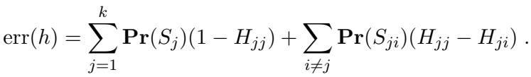
Here, \(S_j\) is the region where the true label is \(j\). The key insight is that if we can create a scenario where the marginal distribution of \(y\) under the “Alternative” hypothesis looks exactly like the “Null” hypothesis, the algorithm gets confused.

Specifically, they look for a condition where the last row of the noise matrix, \(h_k\), is a convex combination of the other rows. This is the mathematical “camouflage.” If the noise profile of class \(k\) looks like a mixture of the noise profiles of classes \(1\) through \(k-1\), the algorithm struggles to tell if it’s looking at class \(k\) or a mix of the others.

Mathematically, if we satisfy this condition, the probability of seeing a label \(y=i\) behaves as follows:

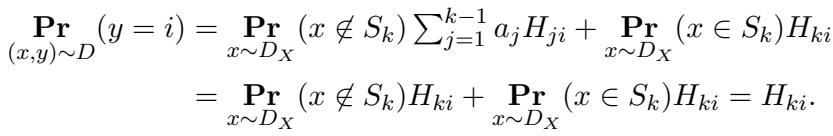
This equation essentially says: “The probability of seeing label \(i\) is \(H_{ki}\) regardless of whether we are in the region \(S_k\) or not.” This completely masks the dependence between \(x\) and \(y\) at the marginal level.

2. Hidden Direction Distributions

To make the testing problem hard, the authors use a technique involving Hidden Direction Distributions.

They assume the data \(x\) is a standard Gaussian in all directions except one specific, secret direction \(v\). Along this direction \(v\), the data follows a specially crafted 1D distribution \(A\).

• In directions orthogonal to \(v\), the data is Gaussian noise.
• The label \(y\) depends only on the projection \(v \cdot x\).

An SQ algorithm needs to “find” \(v\). But if the 1D distribution \(A\) looks very similar to a Gaussian (in terms of its statistical moments), the algorithm has to search through exponentially many directions to find the one where the data isn’t just Gaussian noise.

3. The “Spiky” Marginals

This is where the construction gets clever. The authors need to define regions for the different classes (\(S_1, S_2, \dots\)) along this 1D line.

They define distributions \(A_1, \dots, A_{k-1}\) which correspond to the data distribution given that the ground truth label is \(1, \dots, k-1\).

• These distributions are supported on disjoint intervals (so the classes are separable).
• Crucially, they match the first \(m\) moments of a standard Gaussian distribution.

The figure below illustrates this for \(k=3\).

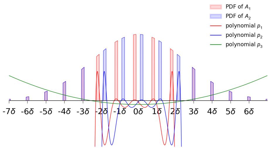
In Figure 1, notice the “spikes” (intervals). The red intervals (\(J_1\)) are where the true label is 1. The blue intervals (\(J_2\)) are where the true label is 2. Everywhere else (the gaps), the true label is 3.

The authors construct these distributions \(A_i\) by taking a Gaussian and slicing it into intervals.

• \(A_1\) is positive on a set of intervals and zero elsewhere.
• \(A_2\) is a shifted version of \(A_1\).
• Outside of the union of these intervals (\(I_{in}\)), the distributions are identical.

By carefully choosing the width and spacing of these intervals, they ensure that \(A_1\) and \(A_2\) have moments that are nearly identical to a standard Gaussian. This means simple statistical statistics (mean, variance, skewness, etc.) cannot distinguish this “spiky” distribution from a smooth Gaussian bell curve.

4. Mixing the Signals

The final piece of the puzzle is how these base distributions translate to the observed noisy data.

Recall the “camouflage” condition: row \(k\) of the noise matrix is a mix of the other rows. When we look at the distribution of data conditioned on the observed label \(y=i\), we get a mixture.

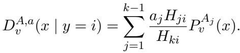
Because the base distributions \(A_j\) are moment-matching Gaussians, any mixture of them is also a moment-matching Gaussian.

The figure below visualizes the conditional distributions \(D|_{y=1}, D|_{y=2}, D|_{y=3}\). Even though the ground truth regions are distinct (the red/blue spikes from Figure 1), the observed distributions conditioned on noisy labels overlap significantly and look “Gaussian-ish.”

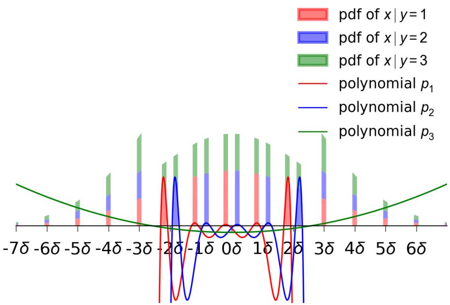
Because these conditional distributions match the moments of a Gaussian, their pairwise correlation is extremely small relative to the Gaussian distribution.

The mathematical bound for the pairwise correlation relies on the chi-squared divergence:

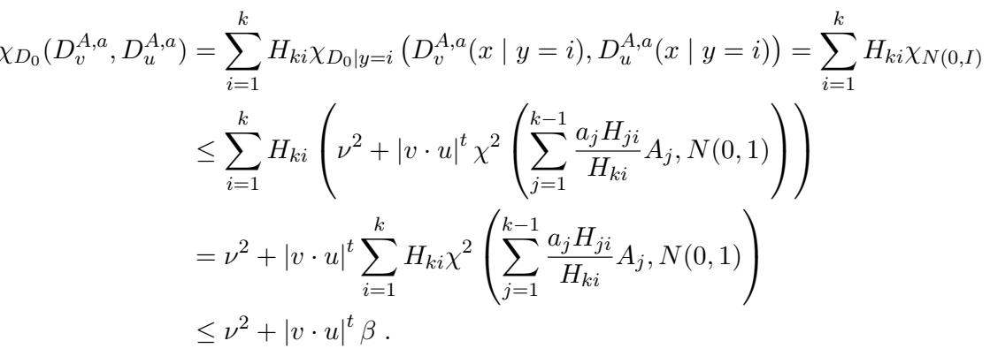
This derivation (Eq 29) essentially proves that the statistical “distance” between the constructed noisy distribution and pure noise is tiny (\(\tau\)). In the SQ model, if the correlation is bounded by \(\beta\) and the query tolerance required is \(\tau\), the number of queries needed scales with the inverse of the correlation. Since the correlation is exponentially small (due to matching many moments), the complexity becomes super-polynomial.

Experiments and Results: The Hardness Theorems

The paper presents three main theoretical results that progressively shut the door on efficient algorithms for MLC with RCN.

Result 1: Hardness of Learning to opt + ε (k=3)

The first result addresses the standard goal of learning: finding a classifier with error close to the optimal possible error (\(\text{opt}\)).

The authors construct a specific \(3 \times 3\) noise matrix \(H\):

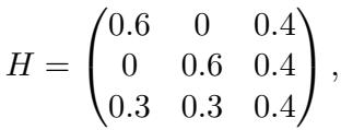
Notice that the third row \((0.3, 0.3, 0.4)\) is exactly the average of the first two rows: \(\frac{1}{2}(0.6, 0, 0.4) + \frac{1}{2}(0, 0.6, 0.4)\). This satisfies the convex combination condition perfectly.

Theorem: For this matrix, any SQ algorithm that learns to error \(\text{opt} + \epsilon\) requires super-polynomial time (specifically \(d^{\tilde{\Omega}(\log d)}\)).

This result is striking because the separation between noise rates (\(\min |H_{ii} - H_{ij}|\)) is a constant (\(0.1\)). Even with well-separated noise, the structure of \(k=3\) allows for this “camouflaging” effect that hides the true classifier.

Result 2: Hardness of Approximation

Perhaps we don’t need the optimal error. Can we just get a classifier that is “good enough”? Maybe within a constant factor of the optimal error?

The authors generalize the construction to larger \(k\). They design a \(k \times k\) matrix where the last row is an average of the first \(k-1\) rows.

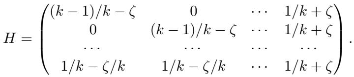
Theorem: For any constant \(C > 1\), there exists a noise matrix (with \(k \approx C\)) such that finding a classifier with error \(C \cdot \text{opt}\) is SQ-hard.

This kills the hope for efficient approximation algorithms. As the number of classes grows, the problem doesn’t just get harder to solve perfectly; it gets harder to solve at all.

Result 3: Hardness of Beating Random Guessing

The final nail in the coffin is the “Random Guessing” lower bound. If you have \(k\) classes and you guess uniformly at random, your error is \(1 - 1/k\). Can we at least do better than that?

The paper shows that for large \(k\) and specific noise matrices (where the “signal” on the diagonal is weak, \(O(1/poly(d))\)), it is SQ-hard to produce a hypothesis with error any better than \(1 - 1/k\).

Implication: In these noisy multiclass settings, complex algorithms might not perform significantly better than a trivial random guesser if they rely on standard statistical queries.

Conclusion

This paper provides a sobering look at the complexity of multiclass classification. It reveals a fundamental discontinuity:

• Binary (\(k=2\)): Noise is a nuisance, but solvable. The geometry of a single hyperplane is robust enough that RCN doesn’t hide the signal entirely.
• Multiclass (\(k \ge 3\)): Noise can mimic the signal. The geometric interplay between multiple decision boundaries and specific noise matrices allows the “noisy” distribution of one class to perfectly simulate the distribution of another class (or a mix of them).

The authors prove that Multiclass Linear Classification with Random Classification Noise is SQ-hard. This suggests that no efficient, noise-tolerant algorithm exists for this problem in the general case without making much stronger assumptions about the data distribution or the structure of the noise matrix.

For students and practitioners, this underscores a vital lesson: intuition from binary classification does not always generalize. The jump from 2 to 3 is not just an increment in numbers; it’s a leap in structural complexity. When dealing with noisy multiclass data, standard linear methods may fail not because the code is wrong, but because the problem itself is fundamentally hard.