](https://deep-paper.org/en/paper/2502.12292/images/cover.png)
In the rapidly expanding universe of Large Language Models (LLMs), provenance has become a messy problem. With thousands of models appearing on Hugging Face every week, a critical question arises: Where did this model actually come from?
Did “SuperChat-7B” actually train their model from scratch, or did they just fine-tune Llama 2 and change the name? Did a startup prune a larger model to create a “novel” efficient architecture, or did they truly innovate?
This isn’t just a question of academic curiosity. It has massive implications for intellectual property, copyright enforcement, and safety auditing. If a model is released with a strict non-commercial license, and another company releases a “new” model that is secretly just a weight-permuted version of the original, how can we prove it?
In a fascinating paper titled “Independence Tests for Language Models,” researchers from Stanford University propose a rigorous statistical framework to answer these questions. They treat model weights not just as numbers, but as evidence in a forensic investigation.
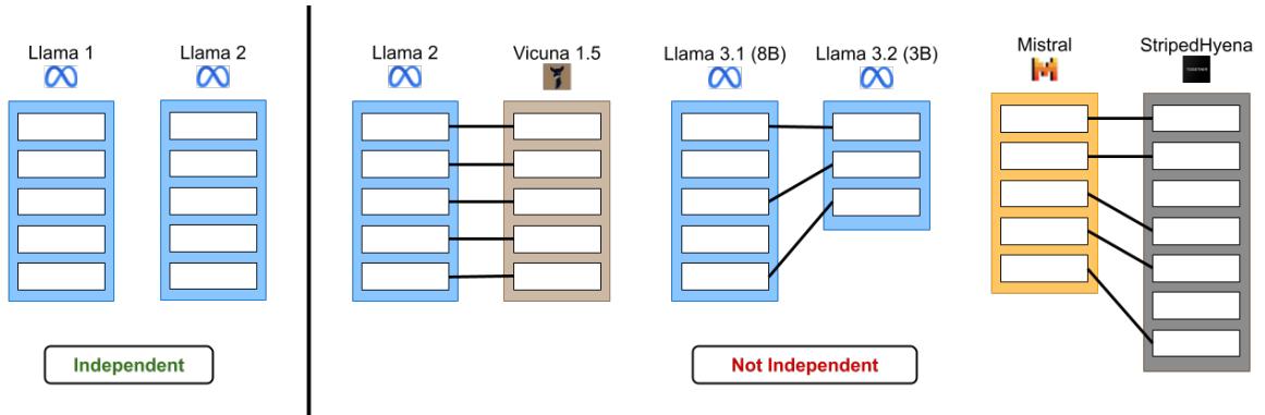
As shown in Figure 1, the goal is to distinguish between models that are truly independent (trained from separate random seeds) and those that share a lineage (fine-tuning, pruning, or merging).
The Core Problem: Defining Independence
To a computer, two neural networks are just two giant lists of numbers (parameters). Even if two models are trained on the exact same dataset with the exact same architecture, if they started with different random seeds (initialization), their final weights will look completely different.
The researchers formulate this as a hypothesis testing problem. The Null Hypothesis (\(H_0\)) is that the two models, \(\theta_1\) and \(\theta_2\), are independent.
\[ H _ { 0 } : \theta _ { 1 } \perp \theta _ { 2 } , \]If we can statistically reject this hypothesis with a low p-value (e.g., \(p < 0.05\) or much lower), we have strong evidence that the models are related.
The paper tackles this in two distinct settings:
- The Constrained Setting: Where we assume the models share an architecture and standard training procedures.
- The Unconstrained Setting: The “wild west” scenario where architectures differ, or an adversary has actively tried to hide the model’s lineage.

Setting 1: The Constrained Setting
Imagine you have two models that look structurally identical—say, both are Llama-7B architectures. You suspect Model B is a fine-tune of Model A.
You might be tempted to just subtract their weights and calculate the Euclidean distance (L2 norm). If the distance is small, they are related, right? Not necessarily. Because neural networks are permutation invariant, this simple distance metric fails.
The Permutation Problem
In a neural network layer, the order of neurons doesn’t matter. You can swap the 5th neuron with the 100th neuron, provided you also swap the corresponding weights in the next layer, and the function remains exactly the same.
If Model B is a fine-tune of Model A, but the developer randomly shuffled the neurons to hide the theft, a simple L2 distance check would show a huge difference, falsely suggesting independence.
The Solution: PERMTEST
The researchers propose a test called PERMTEST. It leverages the fact that standard training algorithms (like SGD or Adam) treat all neurons equally—they are “permutation equivariant.”
Here is the intuition:
- Take Model A.
- Create “fake” copies of Model A by randomly shuffling its hidden units. These copies are statistically identical to Model A under the null hypothesis.
- Compare Model B to Model A.
- Compare Model B to the “fake” shuffled copies of Model A.
If Model B is truly independent of Model A, it should look just as similar (or dissimilar) to Model A as it does to the shuffled copies. However, if Model B is derived from Model A, it will likely be much “closer” to the specific configuration of Model A than to any random shuffling of it.
Evidence: Heatmaps of Provenance
The researchers evaluated this method on the “Llama model tree”—a collection of open-weights models including Vicuna, Alpaca, and others derived from Llama.
They proposed two powerful statistics for comparison:
- \(\phi_{U}\): Comparing the “Up-projection” weights of the MLPs.
- \(\phi_{H}\): Comparing the hidden activations (outputs of neurons) on standard text inputs.
The results were striking. Below is the heatmap for the \(\phi_{U}\) statistic (weights).
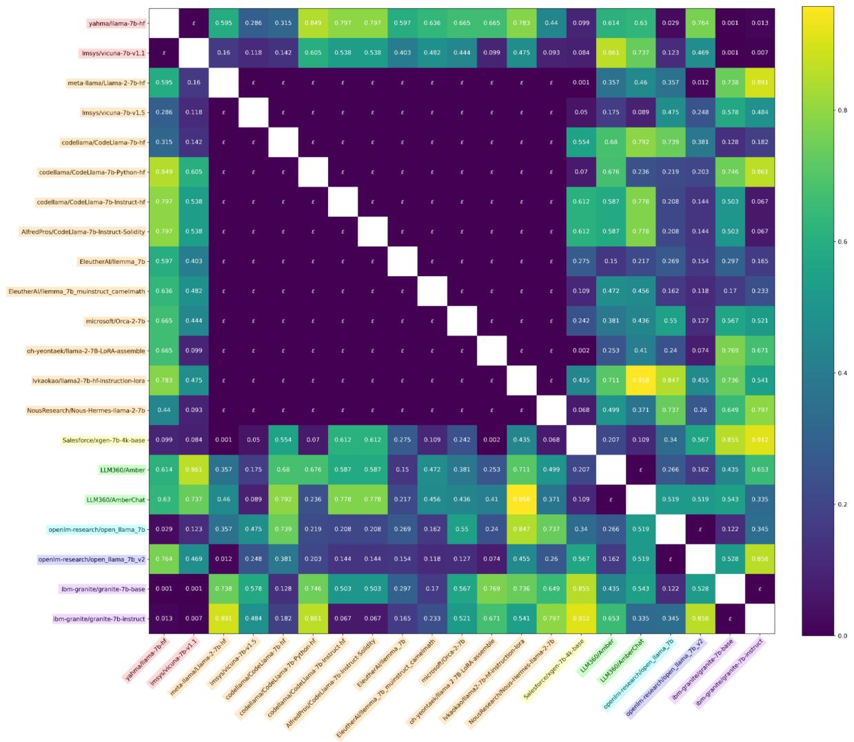
In Figure 7, look at the diagonal. The dark squares represent extremely low p-values (statistical significance). This matrix correctly clusters the “families” of models. For example, all the Llama-2 derivatives light up as dependent on Llama-2, while being independent of the original Llama-1 or unrelated models like OpenLLaMA.
They also found that comparing activations (what the model “thinks”) is often even more robust than comparing weights.
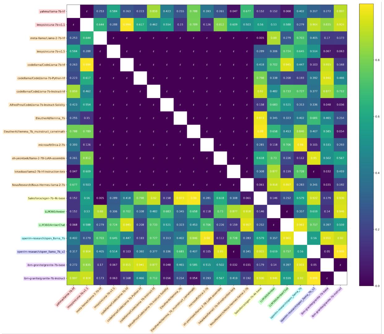
In Figure 8, we see the results using activations. The separation between independent (bright yellow/green) and dependent (dark purple) is incredibly sharp. The researchers were even able to confirm that the leaked “Miqu-70B” model was indeed a quantized version of Llama-2-70B using these tests.
Setting 2: The Unconstrained Setting
The constrained setting is great, but it has a weakness: it assumes we know the architecture, and it breaks if an adversary applies a transformation that PERMTEST doesn’t account for (like a rotation of the feature space).
What if the thief changes the model architecture slightly? Or what if they optimize the model to hide its tracks?
The Robust Test: MATCH + SPEARMAN
To solve this, the authors introduce a robust test based on structural invariants. They focus specifically on the Gated Linear Unit (GLU) MLP, a component used in almost all modern LLMs (Llama, Mistral, etc.).
A GLU MLP has two parallel linear layers: a Gate projection (\(G\)) and an Up projection (\(U\)). They are element-wise multiplied.
\[ f _ { \mathrm { m l p } } ( X _ { \mathrm { L N } _ { 2 } } ^ { ( i ) } ; \boldsymbol { \theta } _ { \mathrm { m l p } } ^ { ( i ) } ) = X _ { i } ^ { \mathrm { M L P } } = [ \sigma ( X _ { i } ^ { \mathrm { L N } _ { 2 } } \boldsymbol { G } _ { i } ^ { T } ) \odot ( X _ { i } ^ { \mathrm { L N } _ { 2 } } \boldsymbol { U } _ { i } ^ { T } ) ] D _ { i } ^ { T } \]The key insight is this: You cannot permute the Gate matrix rows without also permuting the Up matrix rows in the exact same way, or the model breaks.
The researchers devised a statistic called \(\phi_{\text{MATCH}}\).
- Match: They use the Gate matrix (\(G\)) to find the best alignment (permutation) between Model A and Model B.
- Test: They apply that same alignment to the Up matrix (\(U\)).
- Correlate: They calculate the Spearman rank correlation of the aligned Up matrices.
If the models are related, the alignment found via the Gate should also align the Up matrix perfectly. If they are independent, the alignment found on the Gate matrix will be random noise with respect to the Up matrix.
\[ \phi _ { \mathrm { M A T C H } } ^ { ( i , j ) } : = \mathtt { S P E A R M A N } \big ( \mathtt { M A T C H } \big ( H _ { \mathrm { g a t e } } ^ { ( i ) } \big ( \theta _ { 1 } \big ) , H _ { \mathrm { g a t e } } ^ { ( j ) } \big ( \theta _ { 2 } \big ) \big ) , \mathtt { M A T C H } \big ( H _ { \mathrm { u p } } ^ { ( i ) } \big ( \theta _ { 1 } \big ) , H _ { \mathrm { u p } } ^ { ( j ) } \big ( \theta _ { 2 } \big ) \big ) \big ) . \]This test is incredibly robust. It works even if the thief rotates the model weights or changes the hidden dimension size.
Empirical “P-Values”
While this method doesn’t produce theoretically exact p-values like PERMTEST, empirically it behaves exactly like one.

Figure 3 shows that for independent models (the null hypothesis), the distribution of this statistic is uniform (the blue line follows the diagonal). This means valid false positive rates can be controlled.
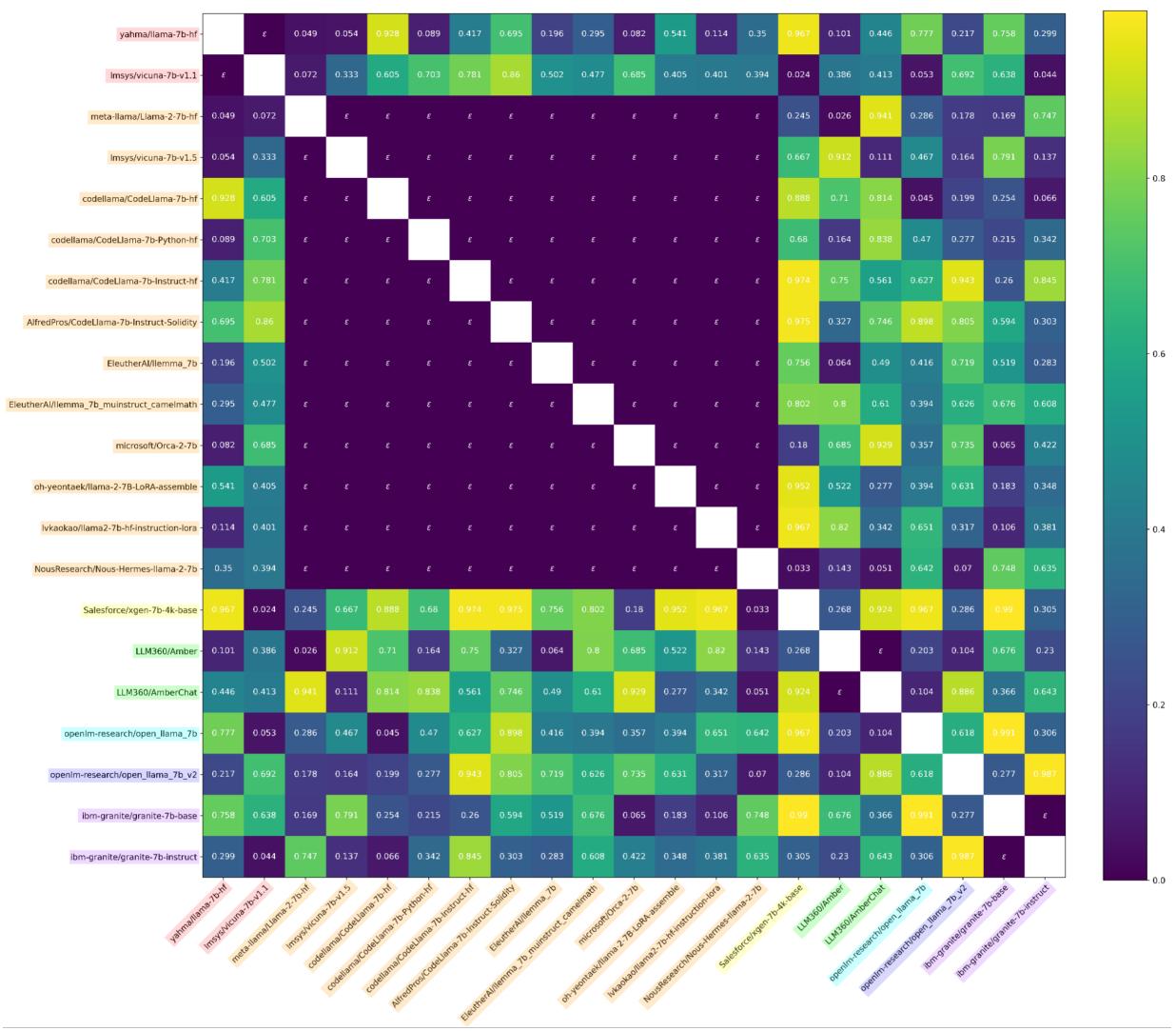
When applied to the model ecosystem, the heatmap again shows clear detection of dependent models, even under adversarial conditions.
Model Forensics: The Case of Llama 3.2
One of the most impressive applications of the Unconstrained Test is Localized Testing. Because \(\phi_{\text{MATCH}}\) aligns specific layers, it can be used to map parts of one model to another.
The authors investigated Llama 3.2 (3B). Meta reported that this model was “pruned” from Llama 3.1 (8B), meaning layers were removed and neurons were deleted to make it smaller. But which layers? And which neurons?
Using their test, the authors matched every layer of the 8B model against every layer of the 3B model.
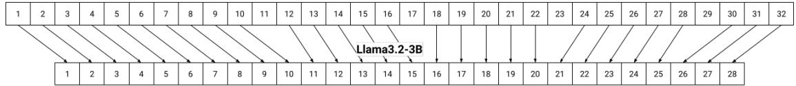
Figure 4 illustrates the discovery. The arrows show exactly which layers from the larger Llama 3.1 (top) correspond to the smaller Llama 3.2 (bottom). You can see that the pruning process kept the early layers (1-6), skipped some middle layers, and kept the final layers. This essentially reverse-engineers the pruning recipe used by Meta.
Furthermore, they analyzed how the neuron dimensions were reduced. Did they just chop off the last 6,000 neurons?
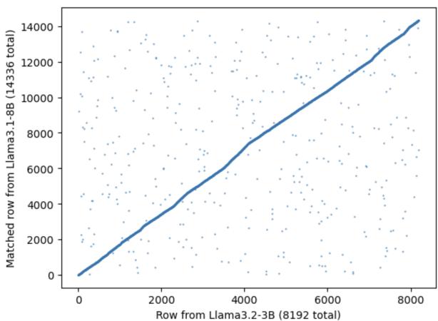
Figure 5 plots the matched neurons. The x-axis is the pruned model indices, and the y-axis is the original model indices. The strong diagonal correlation implies that while many neurons were removed, the ones that remained largely kept their relative ordering and structure.
Defeating the “Strong” Adversary
Finally, the paper addresses a critical counter-argument: “What if I just retrain the layers?”
If a thief steals a model but then re-initializes the MLP layers and retrains them on new data to match the original outputs, surely the weights would drift far enough away to escape detection?
The researchers simulated this. They took a model, ripped out its MLP layers, replaced them with random weights, and retrained them to mimic the original model’s behavior.
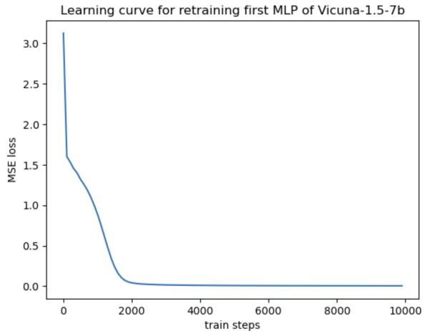
As Figure 10 shows, the loss drops to near zero—the retrained layers are functioning perfectly. However, looking at the test results:
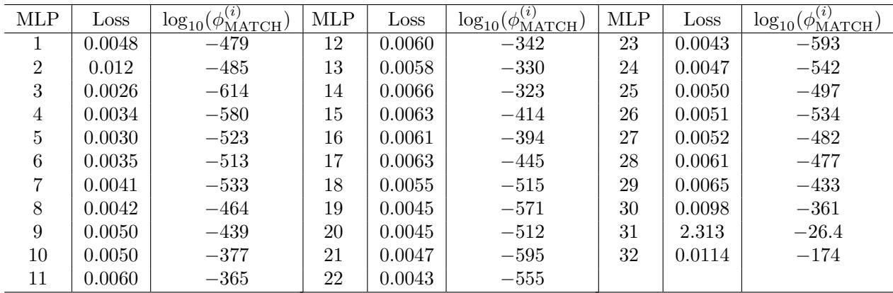
Table 9 reveals that even after this aggressive retraining, the \(\phi_{\text{MATCH}}\) statistic yields p-values like \(10^{-479}\). The models are still overwhelmingly identified as dependent. This suggests that the “shape” of the computation—the functional geometry required to process the data—constrains the weights into a specific basin of attraction that the independence test can detect.
Conclusion
The “wild west” of open weights is becoming a little less lawless. This research demonstrates that hiding the lineage of a Large Language Model is much harder than previously thought.
Whether through direct fine-tuning, pruning, or even adversarial retraining, models carry a statistical fingerprint of their ancestors. By exploiting the permutation invariance of neural networks and the structural constraints of components like GLU MLPs, we can trace these family trees with mathematical certainty.
This toolkit offers a powerful new way for developers to protect their IP and for the community to understand the genealogy of the models driving our AI future.