](https://deep-paper.org/en/paper/2502.14770/images/cover.png)
Introduction
Large Language Models (LLMs) like LLaMA and GPT have revolutionized natural language processing, but they come with a massive cost: their size. With billions of parameters, deploying these models on standard hardware is a logistical nightmare due to high memory footprint and computational latency. This has led to a surge in Network Sparsity research—techniques that aim to remove “unimportant” parameters (weights) from the model to make it smaller and faster without sacrificing intelligence.
Popular post-training sparsity methods, such as SparseGPT and Wanda, have made great strides. They allow us to prune trained models in “one shot” without expensive retraining. However, there is a catch. Most of these methods apply a uniform sparsity rate across the entire network. If you want a 50% sparse model, they remove 50% of the weights from every layer.
But are all layers created equal? Intuitively, no. Some layers handle foundational feature extraction, while others refine high-level concepts.
In this deep dive, we explore a fascinating paper titled “Determining Layer-wise Sparsity for Large Language Models Through a Theoretical Perspective.” The researchers identify a critical phenomenon they call “Reconstruction Error Explosion”—where errors in early layers snowball as they propagate through the network. Their solution, aptly named ATP (A Theoretical Perspective), moves away from complex heuristics and expensive search algorithms. Instead, they derive a mathematically grounded, elegant solution: a monotonically increasing arithmetic progression.
In simple terms: keep the early layers dense and prune the later layers aggressively. Let’s explore why this simple rule works so well.
The Problem: Reconstruction Error Explosion
To understand why standard pruning fails, we first need to understand Reconstruction Error. When we prune a layer (set some weights to zero), the output of that layer changes slightly compared to the original, dense layer. This difference is the reconstruction error.
The goal of any pruning algorithm is to minimize this error. However, existing methods often treat layers in isolation or assume that a uniform cut is “safe enough.” The researchers found that this assumption ignores the cumulative nature of deep neural networks.
The Snowball Effect
The authors propose a theoretical framework that reveals a chain reaction.
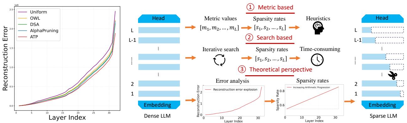
As shown in Figure 1 (Left), look at the “Uniform” (purple) line. The reconstruction error is low in the early layers (indices 0-10) but skyrockets as we get deeper into the network (indices 20-30). This is Reconstruction Error Explosion.
The figure also contrasts the ATP approach with others:
- Metric-based (Heuristic): Using hand-crafted rules (like outlier ratios in OWL) to guess layer importance.
- Search-based: Using evolutionary algorithms (like DSA) to find the best rates, which takes massive compute time.
- ATP (Theoretical): Using a derived mathematical rule (the scissors cutting an arithmetic progression).
Theoretical Proof of Explosion
The paper formalizes this “explosion” through two key theorems.
Theorem 3.1: Sparsity Increases Local Error First, the authors prove that increasing the sparsity of a specific layer always increases the reconstruction error for that layer. If you remove more weights, the approximation gets worse.
The difference in error between a low-sparsity version and a high-sparsity version is quantified as:

In plain English: If you prune more, you break more.
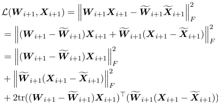
Theorem 3.2: The Cumulative Effect This is the critical insight. The error doesn’t just stay in the layer where it happened. The output of Layer \(i\) becomes the input for Layer \(i+1\). If the input is noisy (due to pruning in Layer \(i\)), Layer \(i+1\) has a harder time reconstructing its original output even if Layer \(i+1\) itself is perfect.
The authors define the reconstruction error for layer \(i\) as:
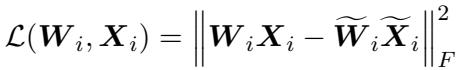
They then prove that the error in the next layer is bounded by the error of the previous layer:
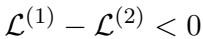
Simplifying this relationship, they arrive at a powerful inequality:

This inequality tells us that error propagates and magnifies. If you damage the first layer of an LLM, you aren’t just hurting Layer 1; you are raising the “error floor” for Layer 2, Layer 3, and so on. By the time the signal reaches Layer 32, the accumulated error has exploded, destroying the model’s ability to reason coherently.
This theoretical analysis leads to a clear strategy: We must prioritize the accuracy of early layers.
The Solution: ATP (A Theoretical Perspective)
If early layers are the most dangerous to prune because their errors propagate furthest, and later layers are safer because their errors have less “distance” to travel, the logical conclusion is a monotonically increasing sparsity rate.
We should prune early layers very little (or not at all) and increase the pruning rate as we go deeper.
The Arithmetic Progression
While we could try to learn a complex curve for this increase, the authors propose using the simplest increasing function: an Arithmetic Progression.
They define the sparsity rate \(s_i\) for layer \(i\) using the following formula:
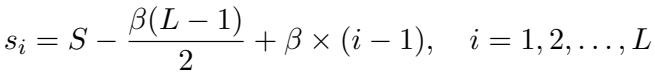
Here is what the variables represent:
- \(s_i\): The sparsity rate for the \(i\)-th layer.
- \(S\): The target average sparsity for the whole model (e.g., 70%).
- \(L\): The total number of layers.
- \(\beta\): The common difference (or slope). This is the only hyperparameter we need to find.
This formula ensures that the average of all layer sparsity rates equals exactly \(S\), while allowing the rates to slope upwards.
Why is this better than Search?
Methods like DSA (Discovering Sparsity Allocation) use evolutionary search to find sparsity rates. This can take days of GPU time and thousands of iterations.
In contrast, the ATP method only requires finding the optimal \(\beta\). Since the sparsity rate must be between 0 and 1, the valid range for \(\beta\) is extremely narrow.
For a LLaMA-7B model with a target sparsity of 70%, the valid range for \(\beta\) is roughly \(0 < \beta \leq 0.019\).
- If \(\beta\) is too high, the first layer’s sparsity drops below 0 (impossible) or the last layer’s exceeds 1.
- The authors use a simple Grid Search with a step size of 0.002.
- This means they only need to check about 9 values.
Instead of searching for days, ATP finds the optimal allocation in roughly 18 minutes on a standard GPU.
Visualizing the Allocation
How does this arithmetic progression compare to other methods?
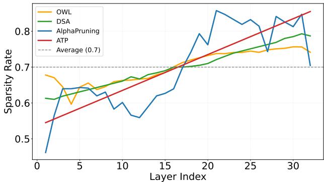
In Figure 3 above, the red line (ATP) starts lower than all other methods (around 40% sparsity) and increases linearly to over 90% at the final layers.
- DSA (Green) and OWL (Orange) fluctuate wildly. They might prune a middle layer aggressively, then spare the next one.
- AlphaPruning (Blue) keeps rates flat and then spikes at the end.
- Uniform (Dashed) is the naive straight line.
The ATP line is smooth and consistent. By starting lower, it preserves the critical early feature extraction, preventing the “error explosion” we saw earlier.
Theoretical Optimality
Is the arithmetic progression just a lucky guess? The authors provide a theorem (Theorem 3.5) proving that a monotonically increasing scheme is strictly better than a non-monotonic one.
They prove this by showing that if you have a pair of layers where the earlier layer has higher sparsity than the later layer (a violation of monotonicity), you can swap their sparsity rates to strictly reduce the total reconstruction error.
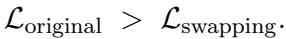
This implies that the optimal distribution must be one where sparsity increases as you go deeper. The arithmetic progression is a robust approximation of this optimal curve.
Experiments and Results
The theory is sound, but does it work in practice? The authors tested ATP on a variety of models (LLaMA, OPT, Vicuna) and tasks.
1. Zero-Shot Accuracy
The most direct test of an LLM’s capability is zero-shot performance on reasoning tasks. Table 1 compares ATP against state-of-the-art methods like OWL, DSA, and AlphaPruning at 70% sparsity.
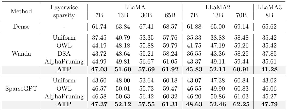
Key Takeaways:
- Significant Gains: On LLaMA-7B, ATP boosts accuracy from 37.45% (Wanda baseline) to 47.03%.
- Beating SOTA: It outperforms the complex AlphaPruning and DSA methods across almost every model size (7B to 70B).
- Consistent Wins: Whether using Wanda or SparseGPT as the base pruner, applying ATP’s layer-wise rates yields the best results.
2. Language Modeling (Perplexity)
Perplexity measures how confused a model is by new text (lower is better). In high-sparsity regimes, perplexity usually spikes.
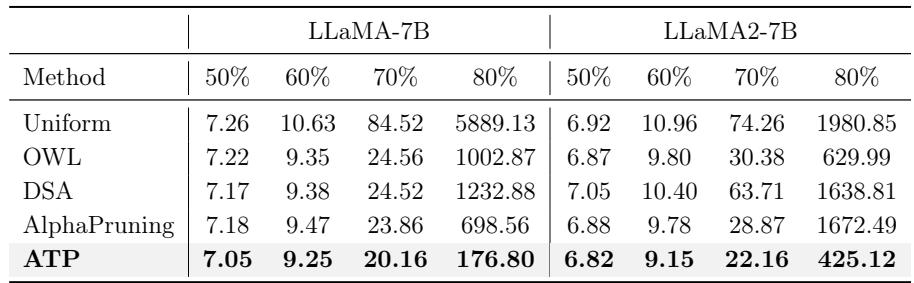
Looking at Table 3, the results at 70% sparsity are striking:
- Uniform: 84.52 (The model is broken).
- OWL: 24.56.
- ATP: 20.16.
At 80% sparsity, the difference is even more dramatic. Uniform sparsity explodes to 5889, while ATP holds steady at 176. This confirms that protecting early layers allows the model to withstand much higher overall compression rates.
3. Comparison with Expensive Search
One might argue that a complex Bayesian search (which explores thousands of combinations) would find a better solution than a simple arithmetic line.
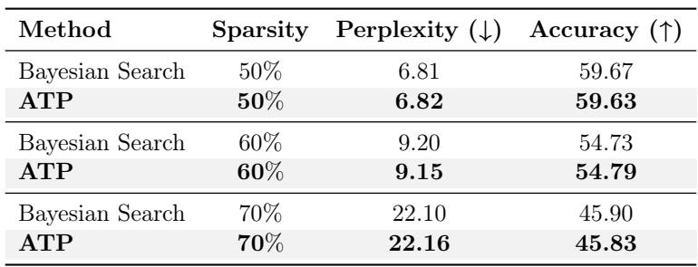
Table 5 reveals a surprising result. ATP matches Bayesian Search.
- At 70% sparsity, Bayesian Search achieves a perplexity of 22.10.
- ATP achieves 22.16.
- The Difference: Bayesian search took 33 hours. ATP took 18 minutes.
This suggests that the “search space” for optimal sparsity is actually quite simple: it just needs to be an upward slope.
4. Real-World Speedup
The ultimate goal of pruning is speed. Does non-uniform sparsity hurt inference speed? (e.g., if one layer is dense, does it become a bottleneck?).
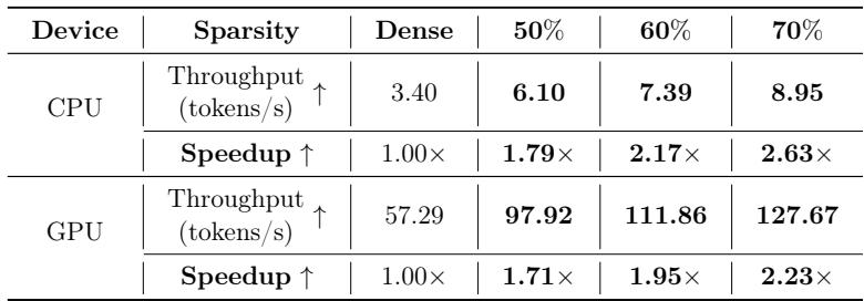
Table 6 shows that ATP provides massive speedups.
- On CPU, a 70% sparse model runs 2.63x faster.
- On GPU, it runs 2.23x faster.
Because the total number of parameters is reduced by 70%, the computational load drops significantly, regardless of the layer-wise distribution.
Finding the Sweet Spot: The Beta Parameter
We mentioned earlier that finding \(\beta\) (the slope) is fast. But does the choice of \(\beta\) matter?
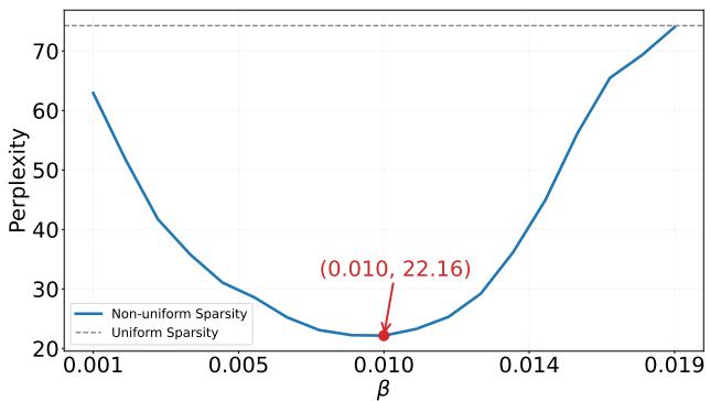
Figure 4 shows the relationship between \(\beta\) and perplexity. It forms a perfect convex “U” shape.
- If \(\beta\) is 0, we have Uniform sparsity (high perplexity).
- As \(\beta\) increases, we slope the sparsity more (protecting early layers), and perplexity drops.
- If \(\beta\) gets too high, we are pruning the final layers too aggressively (near 100%), and perplexity rises again.
This clear convexity explains why Grid Search is so effective—there is a clear global minimum to find.
Conclusion
The paper “Determining Layer-wise Sparsity for Large Language Models Through a Theoretical Perspective” offers a refreshing lesson in AI research: sometimes, theory beats brute force.
By identifying the root cause of performance degradation—Reconstruction Error Explosion—the authors derived a solution that is simpler, faster, and more effective than existing heuristics. The ATP method teaches us that in deep networks, early layers are the foundation. If you crack the foundation, the whole building crumbles. By treating these layers with care and pruning aggressively only at the top, we can compress massive LLMs into efficient, usable models without losing their intelligence.
For students and practitioners, this method is easy to implement. It requires adding just a few lines of code to generate the arithmetic progression mask, yet it yields double-digit percentage gains in accuracy for sparse models. It is a compelling reminder that understanding why a model fails is often more valuable than simply searching for parameters that make it work.