](https://deep-paper.org/en/paper/2502.15988/images/cover.png)
Introduction
In the world of machine learning, there is often a painful trade-off between interpretability (understanding why a model made a prediction) and performance (how accurate that prediction is). Decision trees are the poster child for interpretability. They mimic human reasoning: “If X is true, check Y; if Y is false, predict Z.”
However, building the perfect decision tree—one that is both highly accurate and sparse (few nodes)—is incredibly difficult. This brings us to a second trade-off: optimality vs. scalability.
Historically, you had two choices:
- Greedy Methods (like CART/C4.5): These are lightning-fast. They build trees by making the best immediate decision at every step. However, they are often shortsighted, resulting in larger, less accurate trees.
- Optimal Methods (like GOSDT): These use sophisticated techniques like dynamic programming to find the mathematically perfect tree. They are sparse and accurate but computationally expensive, often taking hours or days to run on complex datasets.
What if you didn’t have to choose?
In the paper “Near-Optimal Decision Trees in a SPLIT Second,” researchers introduce a new family of algorithms—SPLIT, LicketySPLIT, and RESPLIT—that bridges this gap. Their approach produces trees that are practically indistinguishable from optimal ones but runs orders of magnitude faster.
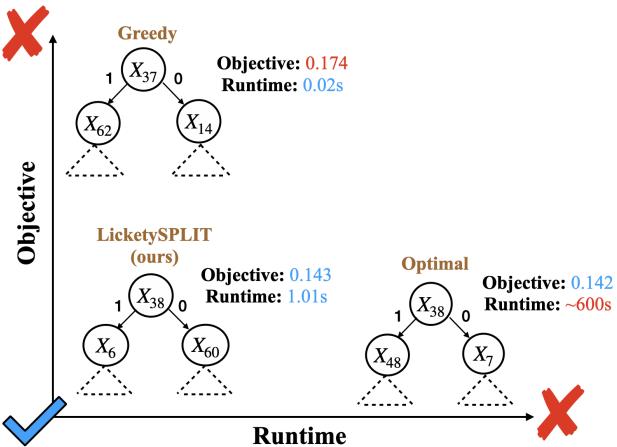
As shown in Figure 1, the proposed algorithm strikes a “perfect balance,” achieving the objective value of optimal methods while maintaining the runtime speed of greedy methods.
The Background: Why is this hard?
To understand the innovation of SPLIT, we first need to look at how decision trees are traditionally built and why “optimal” is so hard to achieve.
The Greedy Trap
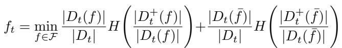
Standard decision tree algorithms are greedy. At the root node, they look at all available features and pick the one that maximizes an immediate metric, such as Information Gain.
Once that split is made, the algorithm never looks back. It repeats the process for the children nodes. The problem is that the “best” split right now might prevent you from making a much better split later deeper in the tree. This myopia often leads to bloated trees that are harder to interpret and generalize poorly.
The Cost of Perfection
Recent years have seen the rise of Optimal Sparse Decision Trees (OSDT). These algorithms solve a global optimization problem. They try to minimize a cost function that penalizes both misclassification error and the size of the tree (number of leaves).
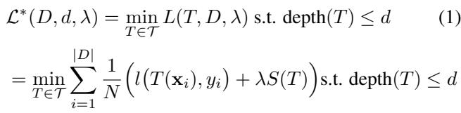
Minimizing this equation (Equation 1) is NP-hard. Algorithms like GOSDT use Branch-and-Bound (BnB) techniques to search the space. They are brilliant but fundamentally limited by the “curse of dimensionality.” As the dataset grows or the tree gets deeper, the number of possible trees explodes exponentially, making optimal search intractable for large problems.
The Rashomon Set
The paper also touches on the concept of the Rashomon Set. In complex problems, there is rarely just one good model. There is usually a set of “good enough” models that perform similarly well.
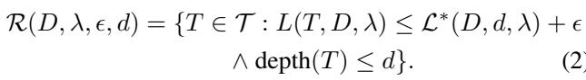
Finding this set (Equation 2) allows users to choose a model that might align better with domain knowledge or fairness constraints. However, finding one optimal tree is hard enough; finding all good trees is even harder.
The Core Insight: Where Optimality Matters
The researchers made a crucial observation that became the foundation of SPLIT: Not all decisions in a tree are created equal.
When building a decision tree, the splits near the root (the top) are the most critical. They partition the entire dataset. A bad decision here ripples down through the entire structure. However, as you go deeper toward the leaves, the sub-problems become smaller (fewer data points).
The researchers hypothesized that while you need powerful optimization for the top of the tree, greedy algorithms perform surprisingly well near the leaves.
They tested this by analyzing optimal trees in the Rashomon set and calculating how often the splits at different depths were “greedy” (i.e., identical to what a simple CART algorithm would choose).
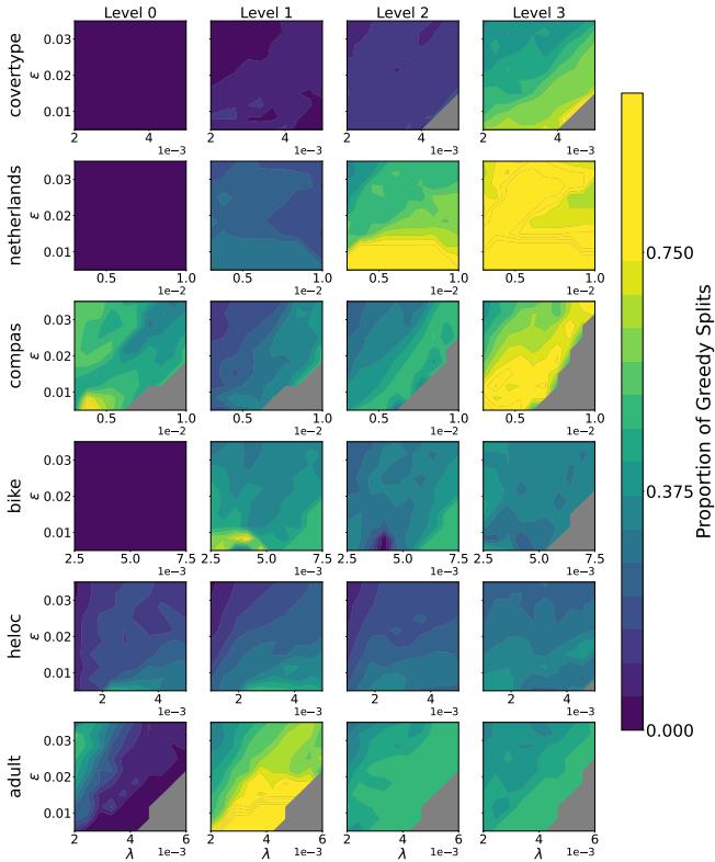
Figure 2 confirms this intuition. At Level 0 (the root), splits are rarely greedy—optimization is required here. But as you approach Level 3 and deeper, the heatmap turns yellow/green, indicating that optimal trees often default to greedy choices near the bottom.
This leads to the guiding principle of SPLIT: Perform a heavy, optimal search near the top, and switch to a fast, greedy search near the bottom.
The Method: SPLIT and LicketySPLIT
The authors propose a “Sparse Lookahead” strategy. Instead of optimizing the entire tree (which is slow) or optimizing none of it (which is inaccurate), they optimize a “prefix” of the tree up to a certain depth.
1. SPLIT Algorithm
The SPLIT algorithm introduces a parameter called lookahead depth (\(d_l\)).
- For the top \(d_l\) layers of the tree, the algorithm uses full Branch-and-Bound optimization to explore all combinations of splits.
- Beyond depth \(d_l\), the algorithm estimates the “cost” of a branch by running a quick Greedy algorithm.
This allows the algorithm to “look ahead” several steps to avoid the traps of pure greedy search, without paying the cost of exploring the entire exponential space of deep trees.
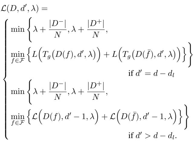
The equation above formally describes this. If the remaining depth \(d'\) allows for lookahead (\(d' > d - d_l\)), it performs the optimal search (the bottom case). Once it hits the lookahead limit, it switches to the greedy approximation (the middle case).
2. LicketySPLIT: Polynomial Time Speed
While SPLIT is fast, the authors introduce an even faster variant: LicketySPLIT.
LicketySPLIT applies the lookahead concept recursively. It essentially runs SPLIT with a lookahead depth of 1 to find the best root split, then recursively calls itself on the left and right children.
Because it breaks the problem down at every step, LicketySPLIT runs in polynomial time (\(O(nk^2d^2)\)), whereas fully optimal methods run in exponential time. This theoretical guarantee is massive: it means LicketySPLIT can scale to datasets where optimal methods would simply crash or run forever.
3. RESPLIT: Fast Rashomon Sets
Finally, they apply this logic to finding the Rashomon set (the set of all good models). RESPLIT uses the SPLIT approach to find a set of “prefix” trees that are promising, and then expands them. This makes the exploration of the “cloud of good models” feasible for high-dimensional data.
Experiments & Results
The theoretical claims are strong, but does it work in practice? The authors compared SPLIT and LicketySPLIT against state-of-the-art optimal algorithms (like GOSDT and MurTree) and greedy baselines.
1. Speed vs. Accuracy Trade-off
The most compelling result is the runtime comparison.
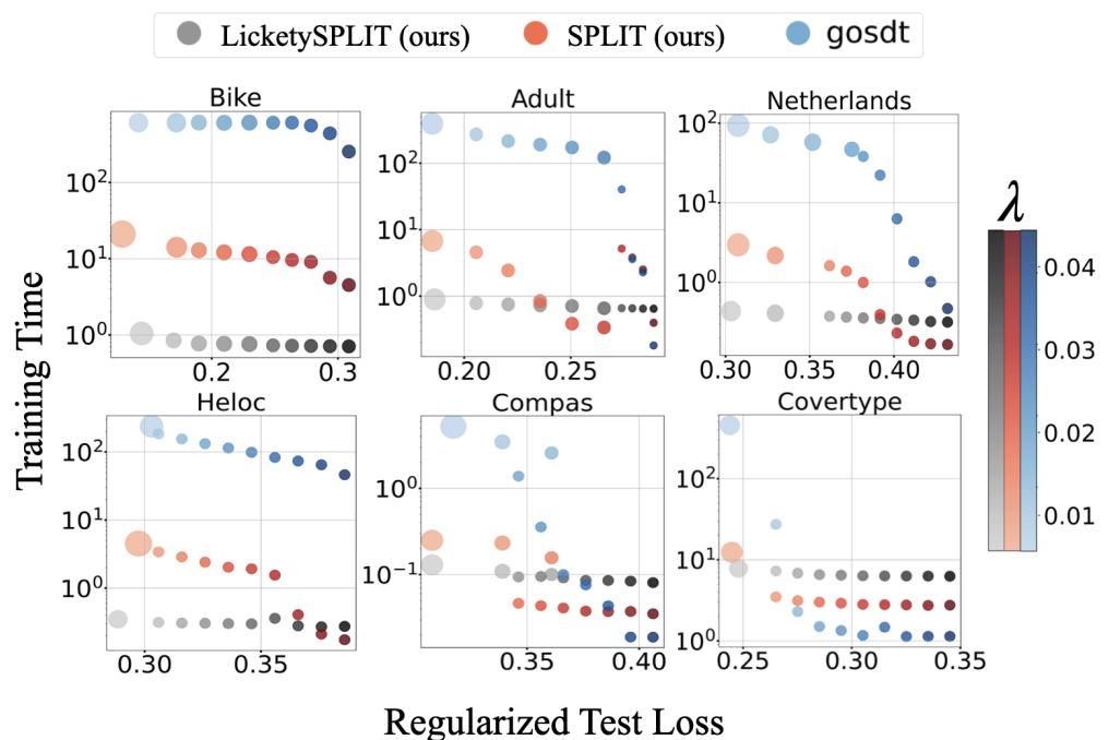
In Figure 3, we see the “Holy Grail” of optimization.
- GOSDT (Blue dots): Achieves low loss but sits far to the right (slow, 100s or 1000s of seconds).
- SPLIT/LicketySPLIT (Red/Grey circles): Sit in the bottom-left corner. They achieve the same low loss as GOSDT but do so in sub-second or single-second times.
On the Bike dataset, SPLIT is roughly 100x faster than the optimal baseline with negligible loss in performance.
2. The Sparsity Frontier
One of the main reasons to use optimal trees is to keep them small (sparse). Do SPLIT trees end up bloated?
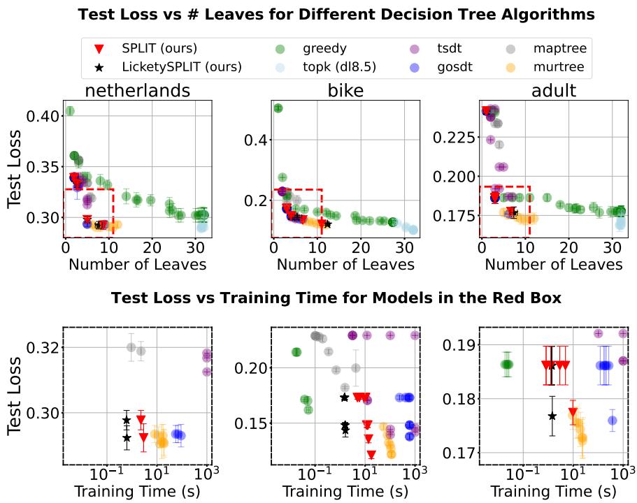
Figure 4 shows the frontier of Test Loss vs. Number of Leaves.
- Greedy trees (Green) are often “high loss, high leaves” (top right of the plots).
- SPLIT and LicketySPLIT (Red/Black stars) land right on top of the optimal solutions (Blue/Yellow). They successfully find the sparse, accurate models located in the “red box” of desirability.
3. How “Optimal” are they?
Are these trees actually optimal, or just close? The authors checked how often the trees produced by SPLIT fell within the Rashomon Set (the set of near-optimal models).
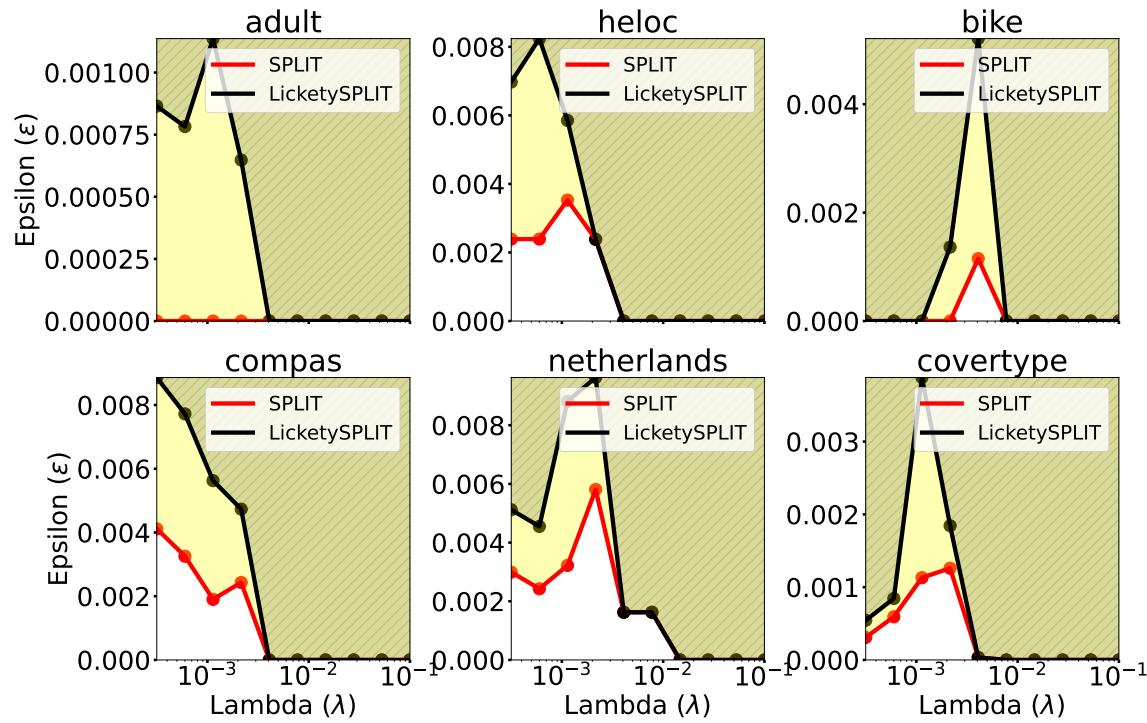
Figure 12 demonstrates that even with very tight constraints (small \(\epsilon\)), the trees generated by SPLIT and LicketySPLIT are essentially optimal. The “optimality gap”—the difference between the perfect tree and the SPLIT tree—is practically non-existent.
4. Lookahead Depth Analysis
A natural question is: “How deep do we need to look ahead?” The authors found that a lookahead depth of roughly \(d/2\) (half the total depth) is theoretically optimal for runtime minimization.
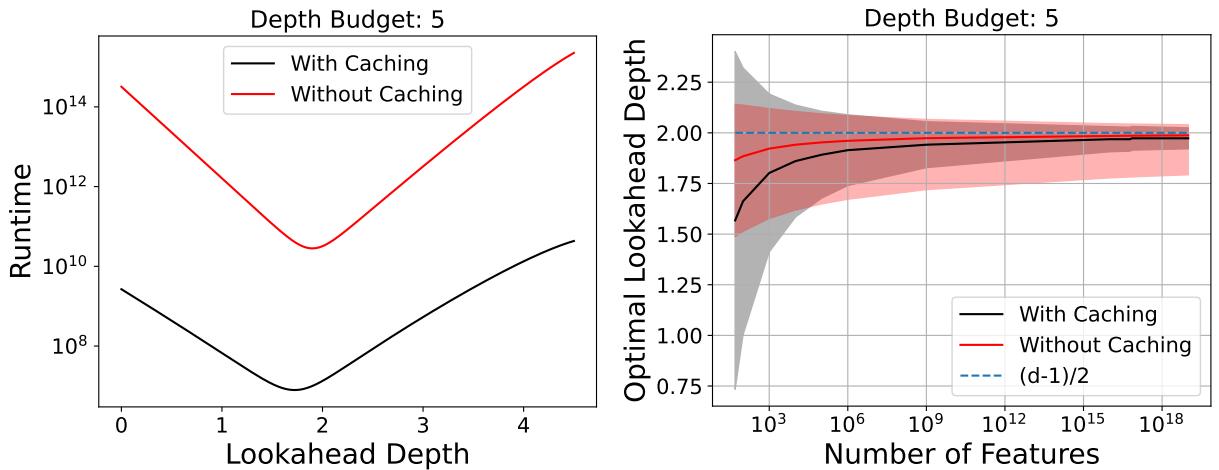
As shown in Figure 19, the runtime forms a “U” shape.
- Too shallow: You rely too much on greedy, potentially making bad choices that require more leaves to fix (or simply failing to find good trees).
- Too deep: You approach the exponential cost of full optimization.
- Sweet Spot: A lookahead of roughly 2 (for depth 5 trees) provides the maximum speedup.
Conclusion
The paper “Near-Optimal Decision Trees in a SPLIT Second” challenges the binary choice between “fast” and “optimal.”
By acknowledging that deep optimization yields diminishing returns near the leaves of a tree, the authors created a hybrid approach. SPLIT and LicketySPLIT leverage the power of Branch-and-Bound where it counts (at the root) and the speed of Greedy search where it’s safe (at the leaves).
Key Takeaways:
- Efficiency: SPLIT is orders of magnitude faster than current state-of-the-art optimal solvers.
- Performance: It sacrifices virtually no accuracy or sparsity.
- Scalability: LicketySPLIT runs in polynomial time, opening the door for optimal-style decision trees on much larger datasets.
This work suggests that for interpretable machine learning, we don’t need to be perfectly optimal everywhere—we just need to be smart about where we optimize.