](https://deep-paper.org/en/paper/2503.01776/images/cover.png)
In the era of Retrieval-Augmented Generation (RAG) and massive vector databases, the quality and efficiency of embeddings—those numerical vector representations of data—are paramount. We want embeddings that are rich in semantic meaning but also lightweight enough to search through millions of records in milliseconds.
For a long time, the industry standard has been dense representations. Recently, Matryoshka Representation Learning (MRL) gained popularity (even being adopted by OpenAI) for its ability to create “nested” embeddings that can be truncated to different lengths. However, MRL comes with a heavy price: it requires expensive full-model retraining and often suffers from significant accuracy drops when the vectors are shortened.
A new paper, “Beyond Matryoshka: Revisiting Sparse Coding for Adaptive Representation,” proposes a compelling alternative. The researchers introduce Contrastive Sparse Representation (CSR), a method that abandons the idea of shortening vectors in favor of making them sparse. By projecting data into a high-dimensional space where only a few “neurons” are active, CSR achieves better accuracy and faster retrieval speeds than MRL, all without needing to retrain the backbone model.
In this post, we will deconstruct how CSR works, the mathematics behind it, and why sparse coding might be the future of adaptive representation.
The Problem: The Trade-off Between Fidelity and Speed
Deep learning models transform inputs (images, text) into fixed-length dense vectors (e.g., 2048 dimensions).
- High dimensions capture more semantic nuance (High Fidelity) but are slow to search (High Latency).
- Low dimensions are fast to search but lose critical information (Low Fidelity).
The Matryoshka Approach (MRL)
MRL attempts to solve this by training a model to order the information within the vector. The most important features are pushed to the front. This allows you to “chop off” the end of the vector (e.g., keep the first 64 dimensions) and still get a decent representation.
However, as shown in Figure 1, MRL (the middle representation) has limitations. To make the first few dimensions powerful, the model compromises the overall quality. Furthermore, you cannot simply apply MRL to an existing model like CLIP or BERT; you have to retrain the whole network from scratch.
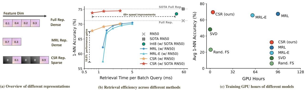
Figure 1(a) illustrates the fundamental difference. MRL relies on short, dense vectors. CSR, the proposed method, uses long vectors but forces them to be sparse—meaning most values are zero. As shown in Figure 1(b), CSR (red stars) achieves higher accuracy with faster retrieval times compared to MRL (blue circles), effectively breaking the usual trade-off curve.
The Solution: Contrastive Sparse Representation (CSR)
The core insight of CSR is that sparsity is a better compression mechanism than truncation. Instead of squeezing information into a tiny dense vector, CSR projects the information into a larger space (e.g., 8192 dimensions) but ensures that for any given input, only a tiny fraction (e.g., 32) of those dimensions are non-zero.
Because the vector is sparse, we don’t need to perform dense matrix multiplication. We can use optimized sparse operations, which scale with the number of non-zero elements (\(K\)) rather than the total dimension (\(d\)).
The Architecture
The CSR framework is a lightweight “adapter” that sits on top of a frozen, pre-trained backbone (like ResNet or a Transformer). This means you can take an off-the-shelf foundation model and make it adaptive without ruining its original weights.
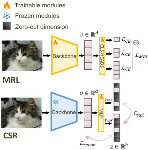
As visualized in Figure 2, the process works as follows:
- Backbone: The image/text passes through a frozen backbone to get a standard dense embedding \(v\).
- Projection (MIP): This vector is projected into a higher-dimensional hidden space.
- Top-K Activation: The system forces a “winner-take-all” dynamic where only the top \(K\) values are kept; the rest become zero.
- Training Objectives: The module is trained using a mix of reconstruction loss (Autoencoding) and discriminative loss (Contrastive).
Let’s break down the mathematical components that make this work.
1. Sparse Autoencoding (SAE)
The first goal of CSR is to ensure the sparse representation retains the information of the original dense embedding. To do this, the authors employ a Sparse Autoencoder.
They use a linear encoder followed by a specific non-linearity called TopK.
The Encoding and Decoding Process:
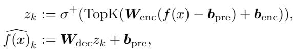
Here, \(f(x)\) is the original dense embedding.
- The encoder projects it to a hidden representation \(z\).
- \(\text{TopK}\) keeps only the \(k\) largest values.
- \(\sigma^+\) is a ReLU activation (ensuring non-negativity).
- The decoder attempts to reconstruct the original input from this sparse \(z_k\).
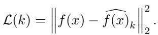
The primary loss function is the Reconstruction Loss, which simply minimizes the distance between the original embedding and the reconstructed version:
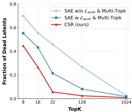
2. Solving the “Dead Latent” Problem
A common failure mode in sparse autoencoders is “dead latents.” This happens when certain dimensions in the hidden space never get activated for any input during training. If a neuron never fires, it’s wasted capacity.
To fix this, the authors introduce a clever auxiliary loss. They calculate the error (residuals) from the main reconstruction and try to reconstruct that error using the “dead” neurons. This forces the model to utilize the entire feature space.
The refined reconstruction objective becomes:

This formula combines:
- Standard reconstruction at sparsity \(k\).
- Reconstruction at sparsity \(4k\) (to encourage a broader set of features).
- An auxiliary loss \(\mathcal{L}_{aux}\) specifically targeting dead latents.
Figure 6 demonstrates the impact of this engineering. The red line (CSR) maintains a near-zero fraction of dead latents, whereas standard SAEs (blue lines) suffer significantly as the sparsity constraint increases.
3. Sparse Contrastive Learning
Reconstruction isn’t enough. For tasks like classification or retrieval, the embeddings need to be discriminative—embeddings of cats should be close to other cats and far from dogs.
MRL handles this by applying Cross-Entropy loss at every truncation level:
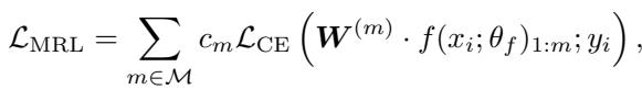
CSR takes a different approach by integrating a Non-negative Contrastive Loss (NCL). This ensures that the sparse features \(z\) are not just good for reconstruction, but also distinct and identifiable.
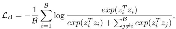
This loss function pushes the sparse representations of positive pairs (e.g., two views of the same image) closer together while pushing negatives apart. Theoretical guarantees suggest that NCL helps disentangle the features, making each dimension in the sparse vector represent a distinct semantic concept.
The Final Objective
The total training objective for CSR combines the reconstruction capability of autoencoders with the discriminative power of contrastive learning:

By balancing these two (\(\gamma=1\) by default), the model creates a representation that is both accurate to the source and useful for downstream tasks.
Why Sparse is Faster (and Better)
One might ask: If the CSR vector is 8192 dimensions, how is it faster than a 2048-dimension dense vector?
The answer lies in Sparse Matrix Multiplication. When calculating the similarity between a query and a database item:
- Dense: You multiply every number by every number. Complexity \(\approx O(d_{dense})\).
- Sparse: You only multiply the non-zero elements. If you enforce Top-32 sparsity, you only perform 32 multiplications, regardless of how large the total dimension \(h\) is. Complexity \(\approx O(K)\).
Figure 3 validates this theory in practice.
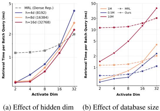
In Figure 3(a), we see that retrieval time is strictly a function of the active dimensions (K). A CSR vector with \(K=16\) retrieves just as fast as an MRL vector of length 16, even though the CSR vector technically exists in a much larger space. Crucially, Figure 3(b) shows that as the database size grows to millions, CSR scales extremely well.
Furthermore, projecting into a higher dimension (\(h\)) helps “unfold” the data manifold, making it easier to separate classes linearly. Figure 5 shows an interesting “Reverse U-shape” behavior:
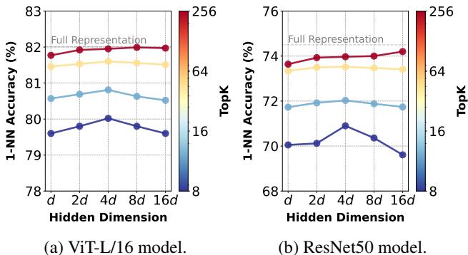
Performance peaks when the hidden dimension is about \(4\times\) the input dimension (\(h=4d\)). This suggests there is a “sweet spot” for expansion before sparsity constraints become too aggressive.
Experimental Results
The paper evaluates CSR across three major modalities: Vision, Text, and Multimodal (Image+Text).
1. Vision: ImageNet Classification
Using ResNet-50 as the backbone, the researchers compared CSR against MRL and other compression techniques (like PCA/SVD).
Figure 7(b) presents the 1-Nearest Neighbor accuracy, a proxy for retrieval performance.
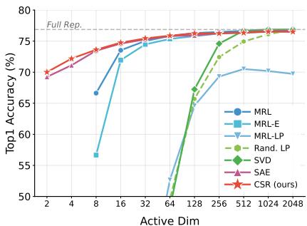
The red line (CSR) dominates the blue line (MRL), especially at the low-dimension end (left side of the x-axis).
- At Active Dimension = 16, CSR creates a usable embedding with high accuracy.
- MRL struggles significantly at these low lengths because it has forcibly engaged in lossy compression.
- CSR matches the “Full Representation” performance (the dashed line) with vastly fewer active parameters.
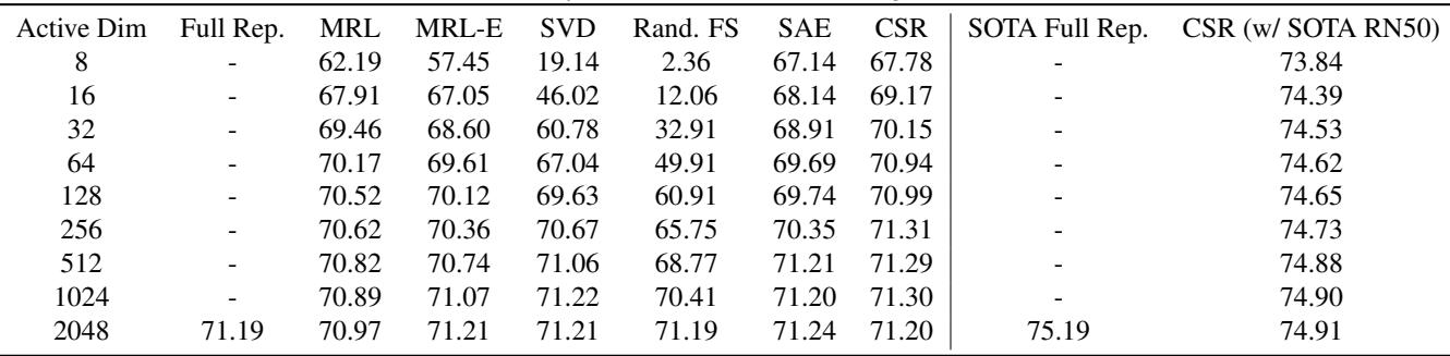
The table below (Table 4) details the exact numbers. Notice how at Active Dim 8, CSR achieves 67.78% accuracy compared to MRL’s 62.19%.
2. Text: MTEB Benchmark
For text embeddings, the authors tested on the Massive Text Embedding Benchmark (MTEB), covering classification, clustering, and retrieval.
The results in Table 1 are striking.
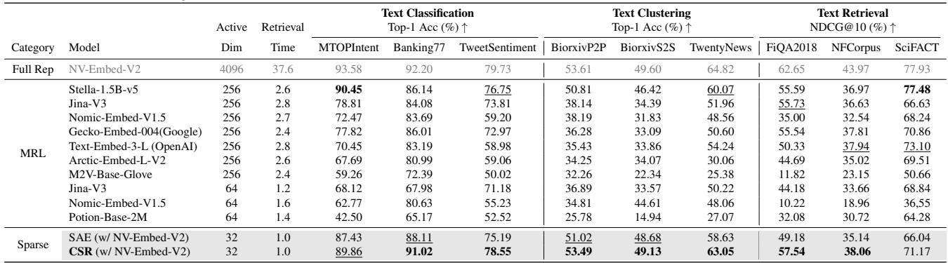
When matching for performance (looking for similar accuracy), CSR offers a 61x speedup in retrieval time compared to the dense baseline. When matching for retrieval efficiency (same speed), CSR provides a 15% performance gain over competitive baselines like Nomic-Embed.
3. Multimodal: Image-Text Retrieval
Finally, they applied CSR to the task of retrieving images using text queries (and vice versa) on MS COCO and Flickr30k datasets.
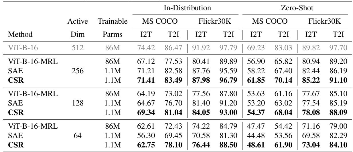
In Table 2, we see that CSR (bolded) consistently outperforms the fine-tuned MRL model. This is particularly impressive because CSR is plug-and-play—it was trained only on the adapter, whereas the MRL baseline involved fine-tuning the heavyweight Vision Transformer (ViT) backbone.
Conclusion: The Case for Sparsity
The “Beyond Matryoshka” paper makes a strong argument that we have been approaching adaptive representation from the wrong angle. Instead of truncating dense vectors—which throws away information and requires re-teaching the model how to pack data—we should be expanding and sparsifying them.
Key Takeaways:
- No Retraining Needed: CSR works on top of frozen, pre-trained models. This saves massive amounts of compute and allows you to upgrade legacy systems easily.
- Better Efficiency Curve: Sparse matrix operations allow CSR to be just as fast as short dense vectors, but with significantly higher accuracy.
- Solved the “Dead Neuron” Issue: Through clever loss engineering, CSR ensures high utilization of the sparse feature space.
As vector databases continue to grow and the demand for low-latency AI increases, techniques like Contrastive Sparse Representation offer a path to have our cake and eat it too: the richness of large models with the speed of tiny ones.
References: Wen, T., Wang, Y., et al. (2025). Beyond Matryoshka: Revisiting Sparse Coding for Adaptive Representation. Proceedings of the 42nd International Conference on Machine Learning.