Introduction

In the world of machine learning, alignment is everything. Whether you are training a generative model to map noise to images, aligning single-cell genomic data across different time points, or translating between distinct domains, you are essentially asking the same question: What is the best way to move mass from distribution A to distribution B?

This is the core question of Optimal Transport (OT). For decades, OT has been the gold standard for comparing and aligning probability distributions because it respects the underlying geometry of the data. It seeks the “least effort” path to transport one dataset onto another.

However, there has always been a massive catch: the “computational wall.” The most popular algorithm for solving OT problems, the Sinkhorn algorithm, scales quadratically. If you double your data, the computation time and memory usage quadruple. For small datasets, this is fine. But in the era of “Big Data”—where we routinely deal with millions of data points—quadratic complexity is a non-starter. It effectively locks the power of OT behind a gate that only small datasets can pass through.

Researchers have tried various workarounds: approximating with mini-batches (which introduces bias) or forcing low-rank constraints (which loses resolution). But what if you could have the best of both worlds? What if you could compute a high-quality, full-rank alignment between millions of points with linear memory and log-linear time?

This is exactly what the paper “Hierarchical Refinement: Optimal Transport to Infinity and Beyond” achieves. The authors introduce a novel algorithm, HiRef, that uses a divide-and-conquer strategy to scale Optimal Transport to levels previously thought impossible. In this post, we will deconstruct how HiRef works, the mathematical insight that makes it possible, and what this means for the future of data alignment.

Background: The Optimal Transport Bottleneck

To understand why HiRef is such a breakthrough, we first need to understand the problem it solves.

The Monge and Kantorovich Problems

Optimal Transport dates back to 1781 with Gaspar Monge, who wanted to move a pile of dirt (source distribution \(\mu\)) to fill a hole (target distribution \(\nu\)) with minimal work. Mathematically, this is known as the Monge Problem. We seek a map \(T\) that pushes \(\mu\) onto \(\nu\) while minimizing the cost \(c\):

Here, \(T(x)\) is the destination of point \(x\). The solution to the Monge problem is a deterministic map—a bijection that pairs every source point uniquely to a target point.

However, a Monge map doesn’t always exist (e.g., splitting one pile of dirt into two holes). This led to the Kantorovich relaxation, which allows mass splitting. Instead of a map, we look for a coupling matrix \(\mathbf{P}\). This matrix describes how much mass moves from \(x_i\) to \(y_j\).

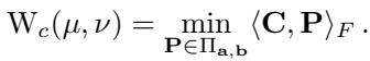
The set \(\Pi_{\mathbf{a}, \mathbf{b}}\) is the collection of all valid coupling matrices where rows sum to the source distribution \(\mathbf{a}\) and columns sum to the target \(\mathbf{b}\). The optimal solution gives us the Wasserstein distance, a powerful metric for measuring the difference between distributions.

The Sinkhorn Algorithm and Its Limits

Solving the standard Kantorovich problem is computationally expensive (cubic time, \(O(n^3)\)). The breakthrough came with the Sinkhorn algorithm (Cuturi, 2013), which added an entropy regularization term \(H(\mathbf{P})\):

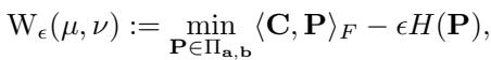
This regularization allows the problem to be solved much faster using simple matrix scaling updates. However, Sinkhorn requires storing and manipulating the \(n \times n\) coupling matrix \(\mathbf{P}\).

If \(n = 100,000\), \(\mathbf{P}\) has \(10\) billion entries. If \(n = 1,000,000\), \(\mathbf{P}\) has \(1\) trillion entries.

This creates a quadratic memory bottleneck (\(O(n^2)\)). For modern datasets with millions of samples (like ImageNet or single-cell transcriptomics), exact OT via Sinkhorn is simply impossible on standard hardware.

Low-Rank Optimal Transport

To bypass the memory issue, researchers developed Low-Rank OT. Instead of storing the full \(n \times n\) matrix \(\mathbf{P}\), they approximate it as the product of smaller matrices with rank \(r\) (where \(r \ll n\)).

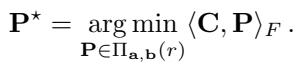
Using a factorization proposed by Scetbon et al. (2021), the coupling is represented as:

Here, \(\mathbf{Q}\) and \(\mathbf{R}\) connect the data to \(r\) “latent” components. This reduces complexity from \(O(n^2)\) to \(O(nr)\), which is linear in \(n\).

The Trade-off: While Low-Rank OT is fast and efficient, it is inherently “blurry.” By forcing the transport plan through a small rank \(r\), you lose the fine-grained, one-to-one correspondence of the Monge map. It groups data points together effectively but cannot tell you exactly which specific point \(x_i\) maps to which specific point \(y_j\).

We are left with a dilemma: Sinkhorn gives high resolution but doesn’t scale. Low-Rank OT scales but loses resolution.

The Core Method: Hierarchical Refinement (HiRef)

The authors of HiRef propose a brilliant way to bridge this gap. Their method assumes that if we zoom in recursively, we can use Low-Rank OT to construct the high-resolution Monge map.

The Key Insight: Co-Clustering

The foundational idea behind HiRef relies on a specific property of Low-Rank OT. When you solve a low-rank problem, the factors \(\mathbf{Q}\) and \(\mathbf{R}\) don’t just compress the data; they cluster it.

Specifically, the authors prove a theoretical result (Proposition 3.1) stating that the factors of an optimal low-rank coupling effectively “co-cluster” points. If point \(x\) in the source dataset maps to point \(y\) in the target dataset under the optimal Monge map, then the low-rank solution will likely assign \(x\) and \(y\) to the same latent component (or cluster).

This observation is the “secret sauce.” It means we can use Low-Rank OT not just as an approximation, but as a sorting mechanism. It tells us: “All these points in Dataset X belong with all those points in Dataset Y. We don’t know the exact pairings yet, but we know they are in the same bucket.”

The Algorithm: Divide and Conquer

HiRef uses this insight to perform a recursive, multiscale refinement.

Step 1: Initialization We start with the two full datasets, \(X\) and \(Y\). We consider this the coarsest scale.

Step 2: Low-Rank Partitioning We solve a Low-Rank OT problem between the current sets. Using the resulting factors \(\mathbf{Q}\) and \(\mathbf{R}\), we partition \(X\) and \(Y\) into \(r\) groups (co-clusters).

The factors \(\mathbf{Q}\) and \(\mathbf{R}\) act as assignment matrices. If row \(i\) of \(\mathbf{Q}\) has its maximum value at column \(z\), then point \(x_i\) is assigned to cluster \(z\). We do the same for \(Y\) using \(\mathbf{R}\). This creates paired subsets: \((X_1, Y_1), (X_2, Y_2), \dots, (X_r, Y_r)\).

Step 3: Recursive Refinement We effectively zoom in. We take the subset pair \((X_1, Y_1)\) and treat it as a new, smaller OT problem. We run Step 2 again on this subset. We do this for all subsets.

Step 4: The Base Case We repeat this process, progressively increasing the resolution (or keeping the rank constant while the dataset size shrinks). Eventually, the partitions become small enough (e.g., single points or very small groups) that we can solve them exactly or they are trivially matched.

At the finest scale, we have established a bijection—a one-to-one map—between the original massive datasets.

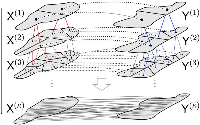
As shown in Figure 1, the algorithm flows from the top (coarse scale) to the bottom (fine scale).

1. Top: The data is one large blob.
2. Middle: Low-rank OT splits the data into matching sub-regions (represented by the red lines connecting specific subsets).
3. Bottom: The process repeats until every point is uniquely paired.

Formalizing the Hierarchy

The algorithm maintains a set of paired partitions, denoted as \(\Gamma_t\) at scale \(t\).

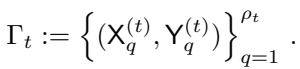
Here, \(\rho_t\) is the total number of clusters at scale \(t\). Each element in \(\Gamma_t\) is a pair of subsets \((X^{(t)}_q, Y^{(t)}_q)\).

At every step of the loop, the algorithm calls a Low-Rank OT solver (LROT) on the currently active partition pair:

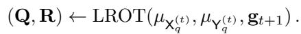
The result creates finer partitions for the next scale \(t+1\).

Theoretical Guarantees

Does this divide-and-conquer strategy actually reduce the transport cost, or does it just chop up the data arbitrarily? The authors provide a proposition (Proposition 3.4) proving that the transport cost decreases (or stays the same) with each refinement step.

They define an “implicit” block coupling \(\mathbf{P}^{(t)}\) at each scale—a matrix we never actually construct in memory, but which conceptually represents the current state of the matching.

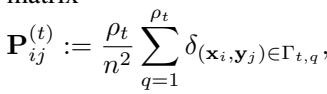
The proposition bounds the change in cost \(\Delta_{t, t+1}\) between refinement levels:

This inequality is crucial. It states that the improvement in cost is bounded by the Lipschitz constant of the cost function \(\|\nabla c\|_\infty\) and the diameter of the partitions. As the algorithm proceeds, the partitions get smaller (\(\mathrm{diam}(\Gamma_{t,q})\) decreases), meaning the solution converges toward the optimal fine-grained mapping.

Complexity: The “Infinity and Beyond” Part

The true beauty of HiRef is its efficiency.

• Space Complexity: Linear (\(O(n)\)). Since we never materialize the full \(n \times n\) matrix, we only store the data and the current partitions.
• Time Complexity: Log-linear (\(O(n \log n)\)) or close to it, depending on the specific rank schedule.

This scaling behavior allows HiRef to handle datasets that would cause a standard Sinkhorn solver to crash immediately.

To maximize efficiency, the authors even formulate an optimization problem to choose the best sequence of ranks \((r_1, r_2, \dots, r_\kappa)\) that factorizes the dataset size \(n\):

This ensures the algorithm performs the minimal amount of work necessary to reach the single-point resolution.

Experiments & Results

The theory is sound, but does it work in practice? The authors benchmark HiRef against Sinkhorn, ProgOT (another scalable solver), and standard Low-Rank methods.

1. Synthetic Benchmarks: Accuracy and Quality

First, they tested the method on synthetic datasets like “Half-Moons” and “S-Curves” to visualize the transport maps.

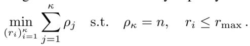
In Figure 2 below, we see the primal OT cost (the total “work” done to move the mass) as a function of sample size.

• Observation: HiRef (blue line) achieves a transport cost almost identical to Sinkhorn (orange) and ProgOT (green). It doesn’t sacrifice quality for speed.
• Scaling: Notice the X-axis. Sinkhorn and ProgOT stop early (around \(10^4\) points) because they run out of memory. HiRef continues comfortably to \(10^6\) (one million) points.

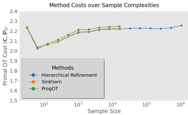
Furthermore, HiRef produces a “hard” bijection (a deterministic map), whereas Sinkhorn produces a “soft” probabilistic coupling. This results in sharper maps.

In Figure 3, compare the Hierarchical Refinement Map (top row) with the Sinkhorn Barycentric Map (middle row).

• The Sinkhorn map often pulls points toward the “average” (barycenter), causing the target shape to shrink or look warped (notice the gap in the S-curve in row a).
• The HiRef map maintains the geometry of the target distribution much more faithfully, looking very similar to the ground-truth optimal map (bottom row).

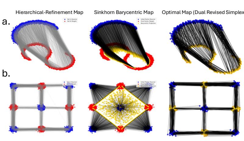
2. Massive Biological Datasets: Mouse Embryogenesis

Optimal Transport is heavily used in biology to reconstruct developmental trajectories—figuring out how cells evolve over time. The authors applied HiRef to a massive spatiotemporal transcriptomics dataset of mouse organogenesis (MOSTA).

They aligned cells between developmental time points (e.g., Day 13.5 to Day 14.5). These datasets contain hundreds of thousands of cells.

Table 1 shows the transport costs.

• Sinkhorn: Fails (Out of Memory) for all large stages.
• HiRef: Successfully runs on all pairs.
• Performance: HiRef consistently achieves lower transport costs (lower is better) compared to Mini-Batch (MB) approximations. For example, in the E15-16.5 transition, HiRef achieves a cost of 12.79 compared to 12.91 for large-batch OT.

3. Spatial Alignment: MERFISH Brain Atlas

In another biological experiment, they aligned slices of a mouse brain based solely on spatial coordinates and then checked if the gene expression matched up. This is a rigorous test: if the spatial alignment is wrong, the biology won’t match.

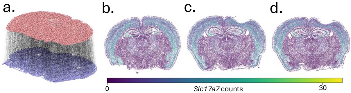
Figure 4 visualizes the results.

• a: The 3D alignment of the brain slices.
• b, c, d: The gene expression of Slc17a7.
• (b) is the source.
• (d) is the true target.
• (c) is the predicted target using the HiRef mapping.
• Result: The predicted map (c) looks nearly identical to the ground truth (d), with a cosine similarity of 0.8098. Standard Low-Rank methods (like FRLC) struggled here, achieving much lower similarity scores (around 0.23). This proves that the refinement aspect of HiRef is necessary to capture fine-grained local structure.

4. The Million-Image Challenge: ImageNet

Finally, the ultimate scalability flex. The authors aligned 1.28 million images from the ImageNet dataset (represented as 2048-dimensional embeddings).

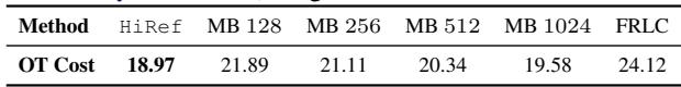
Table 2 tells the story.

• Sinkhorn / ProgOT / LOT: Could not run (Memory/Time constraints).
• HiRef: Completed the task with a cost of 18.97.
• Mini-Batch (MB): Even with large batch sizes (1024), the cost was higher (19.58), indicating a worse alignment.

HiRef successfully computed a full-rank alignment between two datasets of over a million points each—a feat previously considered impractical for global Optimal Transport.

Conclusion & Implications

The paper “Hierarchical Refinement” presents a significant leap forward for computational Optimal Transport. By combining the speed of low-rank approximations with a recursive, multiscale strategy, the authors have effectively dismantled the quadratic barrier that held OT back.

Key Takeaways:

1. Low-Rank factors are clusters: The algorithm leverages the mathematical property that low-rank OT factors naturally group corresponding source and target points.
2. Refinement recovers resolution: By recursively solving smaller sub-problems, HiRef recovers the fine-grained Monge map that standard low-rank methods smooth over.
3. Scalability is solved: With linear space and log-linear time, OT can now be applied to datasets with millions of samples without relying on biased mini-batching.

Why does this matter? This opens the door for using “true” Optimal Transport in deep learning areas that were previously restricted to approximations. We could see better generative models (aligning noise to data more accurately), more precise biological trajectory inference (tracking millions of cells), and improved domain adaptation in computer vision.

HiRef turns the “curse of dimensionality” into a divide-and-conquer opportunity, proving that with the right hierarchy, we really can take Optimal Transport to infinity and beyond.

This blog post explains the research paper “Hierarchical Refinement: Optimal Transport to Infinity and Beyond” by Halmos et al. (2025).