](https://deep-paper.org/en/paper/2503.17061/images/cover.png)
Imagine a smart drone deployed to monitor a remote wildlife sanctuary. Initially, it’s trained to recognize eagles and deer. But one day, a new species—a fox—moves into the area. For the drone to remain useful, it must learn to identify this new animal without forgetting what an eagle or deer looks like. This ability to learn sequentially, without losing past knowledge, is called Continual Learning (CL).
For artificial intelligence systems, this is a surprisingly hard problem. When a standard neural network learns something new, it often overwrites its old knowledge—a phenomenon known as catastrophic forgetting (CF). As shown in Figure 1, while the model’s accuracy on the new task rises sharply, its performance on previous tasks drops dramatically.
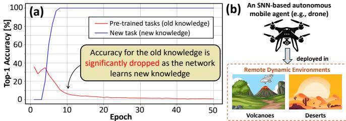
Figure 1. Panel (a) shows catastrophic forgetting, where accuracy on old tasks (red line) drops as the model learns a new task (blue line). Panel (b) illustrates the target application: an autonomous drone that requires efficient continual learning in remote environments.
Retraining the entire model from scratch with both old and new data is a brute-force solution—but one that’s infeasible for embedded or resource-constrained systems. It demands enormous time, energy, and access to complete datasets, which is often restricted due to storage or privacy concerns. This is especially problematic for small, battery-powered devices like drones or robots operating at the edge.
This is where Spiking Neural Networks (SNNs) come in. Inspired by the human brain, SNNs communicate via discrete, energy-efficient “spikes,” making them ideal for low-power systems. The pursuit of continual learning within SNNs forms the basis of a growing research field called Neuromorphic Continual Learning (NCL).
A recent study, Replay4NCL: An Efficient Memory Replay-based Methodology for Neuromorphic Continual Learning in Embedded AI Systems, tackles this challenge head-on. The authors introduce Replay4NCL, a novel technique that not only prevents catastrophic forgetting but does so with remarkable efficiency, ushering in a new era of adaptive edge AI.
The Problem with “Remembering” in AI
One proven strategy to fight catastrophic forgetting is memory replay. The idea: while an AI learns new information, it periodically “replays” compact representations of old tasks. This helps the system reinforce prior knowledge and prevent it from being overwritten.
The state-of-the-art method for SNNs, called SpikingLR, uses such memory replay. However, it’s ill-suited for embedded applications—it’s slow and power-hungry. To maintain high accuracy, SpikingLR relies on long processing durations called “timesteps,” similar to frames in a slow-motion video. More timesteps mean more computation, increasing latency and energy consumption.
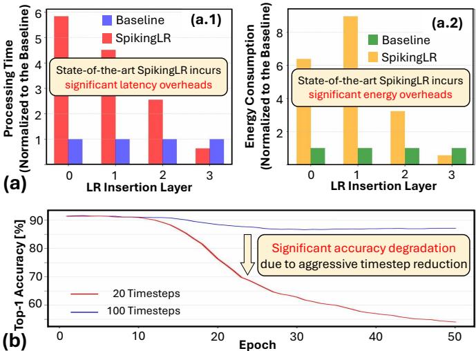
Figure 2. Panel (a) shows that the state-of-the-art SpikingLR method incurs significant latency and energy overheads. Panel (b) demonstrates that simply reducing timesteps from 100 to 20 leads to severe accuracy loss.
As seen above, SpikingLR introduces heavy computational overheads. Naively cutting down on timesteps leads to major information loss and degraded performance. Thus, the Replay4NCL work addresses a critical question: How can memory replay be made efficient enough for embedded AI without sacrificing accuracy?
A Quick Primer: Spiking Neural Networks and How They Learn
Spiking Neural Networks (SNNs)
Unlike conventional neural networks that handle continuous signals, SNNs process discrete events—spikes, akin to biological neurons. A neuron’s internal state, known as the membrane potential (\(V_{mem}\)), rises as it receives spikes. Once it crosses a threshold (\(V_{thr}\)), the neuron emits a spike and resets.
This behavior is captured in the Leaky Integrate-and-Fire (LIF) model:
\[ \tau \frac{dV_{mem}(t)}{dt} = -(V_{mem}(t) - V_{rst}) + Z(t) \]Here, \(V_{rst}\) is the reset potential, \(Z(t)\) represents inputs, and \(\tau\) sets the decay rate of the potential.
If \(V_{mem} \ge V_{thr}\), the neuron fires, resetting its potential:
\[ V_{mem} \leftarrow V_{rst} \]This event-driven computation yields sparse and highly efficient processing—perfect for embedded systems.
Training SNNs with Surrogate Gradients
Training SNNs is complex since the “spike” activation isn’t differentiable—making standard backpropagation impossible. The breakthrough came through Surrogate Gradient (SG) learning, which replaces the non-differentiable step function with a smooth, differentiable curve during backpropagation.
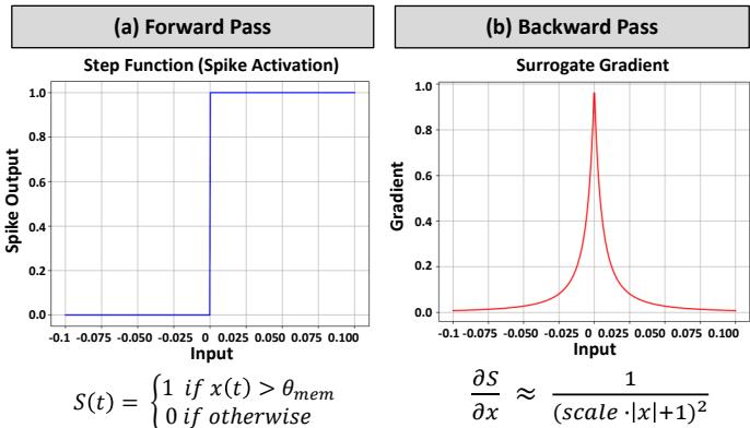
Figure 5. The forward pass (a) uses a non-differentiable step function for spike activation. During training, a smooth “surrogate gradient” (b) allows gradient-based optimization.
This technique allows gradients to propagate even through spiking activations, enabling powerful supervised training of SNNs.
The Replay4NCL Methodology: Three Steps to Efficiency
The Replay4NCL approach introduces three key innovations, summarized in Figure 4. Together, they drastically reduce latency and energy while preserving learning quality.
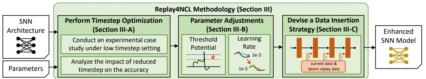
Figure 4. The Replay4NCL process consists of three coordinated steps: Timestep Optimization, Parameter Adjustments, and Data Insertion Strategy design.
Let’s unpack each step.
Step 1: Perform Timestep Optimization
The most direct path to low latency and energy consumption is to reduce timesteps. But as earlier results (Figure 2) show, aggressive reductions destroy accuracy. The goal is to find a balance—fast yet precise.
Researchers conducted experiments to explore this trade-off between timesteps, accuracy, and processing time.
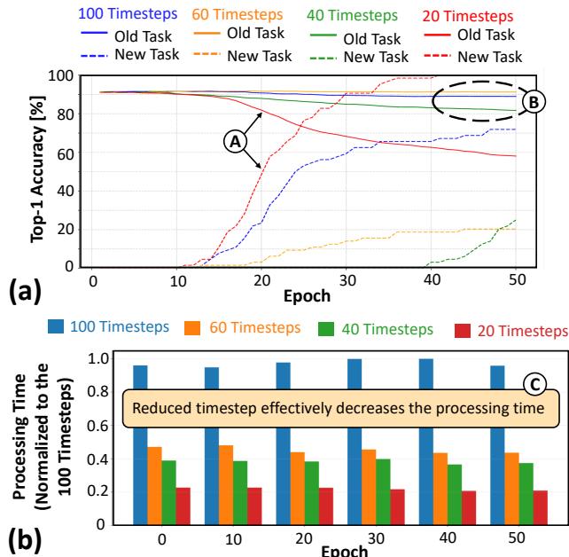
Figure 8. (a) Reducing timesteps from 100 to 20 severely hurts accuracy, while 40 timesteps offer a good compromise. (b) Processing time decreases dramatically with fewer timesteps.
They found that 40 timesteps maintain high accuracy while sharply reducing processing time—striking the right balance for embedded systems.
Fewer timesteps also mean smaller latent replay data (snapshots of neurons when recalling old tasks). To make this replay data even more storage-efficient, Replay4NCL employs a simple compression-decompression scheme.
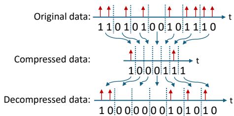
Figure 7. The lossless compression and decompression mechanism efficiently stores and retrieves latent replay data.
Timestep optimization and compression together minimize both latency and memory footprint.
Step 2: Perform Parameter Adjustments
With fewer timesteps, neurons fire fewer spikes. This limits information flow, which can hinder learning. Replay4NCL counters this by adjusting two crucial parameters.
- Neuron Threshold Potential (\(V_{thr}\)) — Reduced slightly so neurons fire more easily despite fewer inputs.
- Learning Rate (\(\eta\)) — Lowered to allow gentler weight updates when information is sparse.
This balancing act keeps the spiking activity consistent with the pre-trained model, enabling smooth adaptation to a low-timestep regime.
Step 3: Devise a Data Insertion Strategy
The final piece concerns where and how to inject latent replay (LR) data. The SNN architecture, shown in Figure 6, divides its layers into frozen (unchanged) and learning (updated) parts. LR data is inserted at the boundary between these layers.
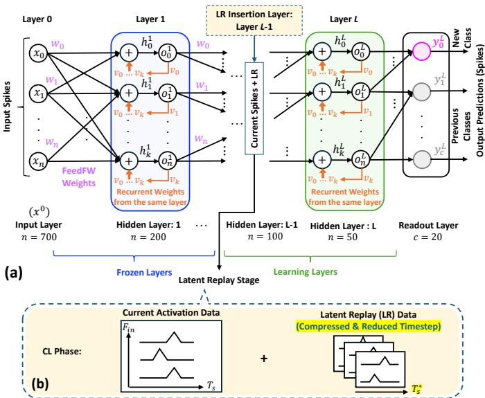
Figure 6. The SNN is split into frozen and learning layers. Latent replay data is injected at strategic layers to reinforce prior tasks during new learning.
Replay4NCL dynamically explores different insertion layers and introduces a threshold adaptation mechanism. During training, the neuron threshold (\(V_{thr}\)) adjusts based on spike timing—rising or falling smoothly to maintain balance. In combination with a reduced learning rate, this ensures robust, stable learning from both old and new tasks.
In practice, the training process unfolds in three stages:
- Pre-training: Learn initial tasks and develop stable weights.
- Preparation: Generate compressed replay data using optimized timesteps and adaptive thresholds.
- Continual Learning: Train on new tasks using both fresh and replayed data, with dynamic thresholds and reduced learning rate.
Testing Replay4NCL: The SHD Benchmark
The authors evaluated Replay4NCL on the Spiking Heidelberg Digits (SHD) dataset—a common benchmark for neuromorphic audio signals. The setup (Figure 9) used a Python-based implementation running on an Nvidia RTX 4090 Ti GPU.
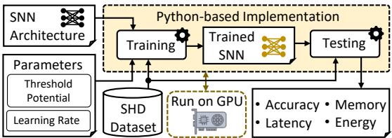
Figure 9. Python-based evaluation pipeline using GPU acceleration and the SHD dataset to assess accuracy, memory, latency, and energy.
The test scenario simulated incremental learning: train on 19 sound classes, then learn the 20th without losing the previous 19.
Results: Faster, Lighter, and Smarter
Accuracy: No Compromises
Replay4NCL achieves accuracy comparable to—and sometimes exceeding—the state-of-the-art SpikingLR.
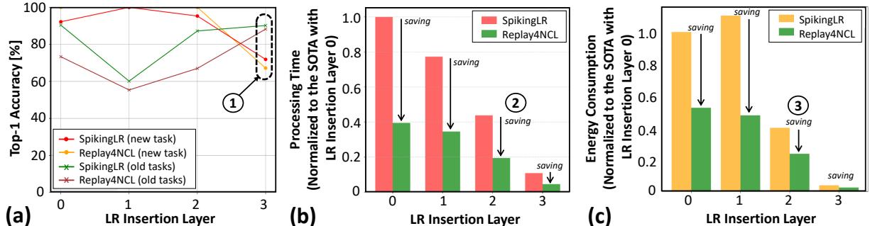
Figure 10. (a) Replay4NCL (green) matches or surpasses SpikingLR (red/orange) in accuracy while offering (b) major latency reductions and (c) substantial energy savings.
In the optimal configuration (LR insertion layer 3), Replay4NCL maintains higher accuracy on old tasks than SpikingLR, as seen below.
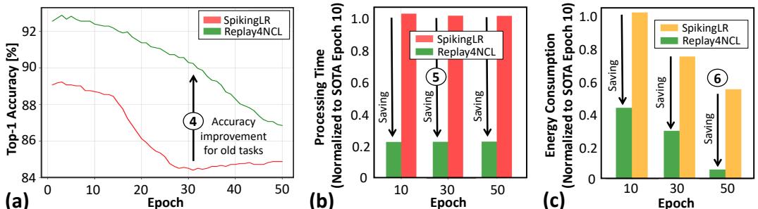
Figure 11. At LR insertion layer 3, Replay4NCL achieves better accuracy for old tasks (a), while being faster (b) and more energy-efficient (c) across epochs.
Latency, Memory, and Energy: Massive Gains
Replay4NCL’s optimized timestep turns into performance gold:
- 4.88× faster processing latency
- ~20% memory savings for storing replay data
- 36.43% lower energy consumption
These improvements make it ideal for real-time and battery-sensitive systems.
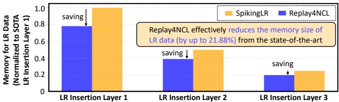
Figure 12. Replay4NCL requires less memory to store replay data than SpikingLR, saving up to 21.88%.
The reduction in time directly translates into lower energy use—a crucial advantage for mobile or autonomous agents.
Learning Stability: Long-Term Consistency
Replay4NCL also shines in long-term learning. Extending training to 150 epochs revealed smoother, more stable convergence, unlike the volatile behavior of SpikingLR.
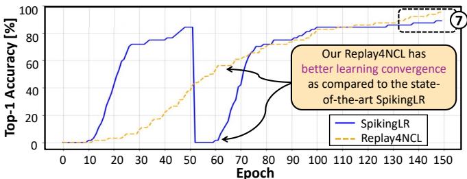
Figure 13. Over 150 epochs, Replay4NCL (orange dashed line) shows smoother, more stable learning convergence than the fluctuating SpikingLR (blue line).
This stability means Replay4NCL not only learns efficiently—it learns reliably.
Conclusion: A Leap Forward for Embedded AI
Catastrophic forgetting has long hindered the goal of truly adaptive AI. While memory replay mitigates it, prior methods were too computationally intensive for edge devices.
Replay4NCL delivers an elegant, practical solution. By combining timestep optimization, parameter calibration, and strategic data replay, the approach achieves continual learning that’s both robust and energy-efficient.
Replay4NCL preserves old knowledge with 90.43% Top-1 accuracy, outperforms the state-of-the-art by 4.88× in latency, and cuts memory and energy demands by 20% and 36.43%, respectively.
This methodology marks a major step toward intelligent systems that learn and adapt over time—without draining resources. With Replay4NCL, embedded AI can finally learn not just once, but for life.