Seeing How They Think: Unlocking Neural Network Dynamics with Manifold Geometry

How does a neural network actually learn?

If you look at the raw numbers—the billions of synaptic weights—you see a chaotic storm of floating-point adjustments. If you look at the loss curve, you see a line going down. But neither of these tells you how the network is structuring information.

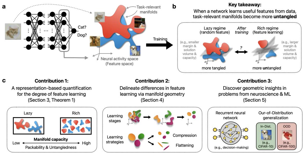
For a long time, researchers have categorized deep learning into two distinct regimes: the Lazy regime and the Rich regime. In the lazy regime, the network barely touches its internal features, acting like a glorified kernel machine. In the rich regime, the network actively sculpts complex, task-specific features.

But this binary view is too simple. It’s like classifying all transportation as either “walking” or “sprinting,” ignoring everything from bicycles to airplanes. Feature learning is a spectrum, full of nuanced strategies and distinct stages.

In this post, we will explore a new analytical framework presented in Feature Learning beyond the Lazy-Rich Dichotomy, which uses Representational Geometry to peer inside the “black box.” By modeling data as geometric manifolds (clouds of points) moving through high-dimensional space, we can visualize exactly how neural networks untangle complex problems—and why they sometimes fail to generalize.

Part 1: The Problem with “Lazy vs. Rich”

To understand the contribution of this work, we first need to understand the current prevailing theory.

The Lazy Regime

Imagine a neural network where the internal layers are initialized randomly and stay fixed. Only the final layer (the classifier) updates its weights to solve the task. This is essentially how “Lazy Learning” works. The network doesn’t learn new features; it just figures out how to combine the random features it started with. Mathematically, this behaves like a Kernel method (specifically, the Neural Tangent Kernel or NTK).

The Rich Regime

In contrast, modern deep learning usually operates in the “Rich Regime.” Here, the internal weights change significantly. The network learns to detect edges, then textures, then object parts. It builds a hierarchy of features optimized for the specific task at hand.

The Gap

Researchers have developed metrics to guess which regime a network is in, such as tracking the distance weights move from initialization. However, these metrics are proxy measurements. They look at the mechanism (weights) rather than the outcome (representation). They often fail to distinguish between different “flavors” of rich learning or explain why a network might learn well but fail to generalize to new data (Out-of-Distribution).

We need a way to measure the quality and structure of the learned features directly.

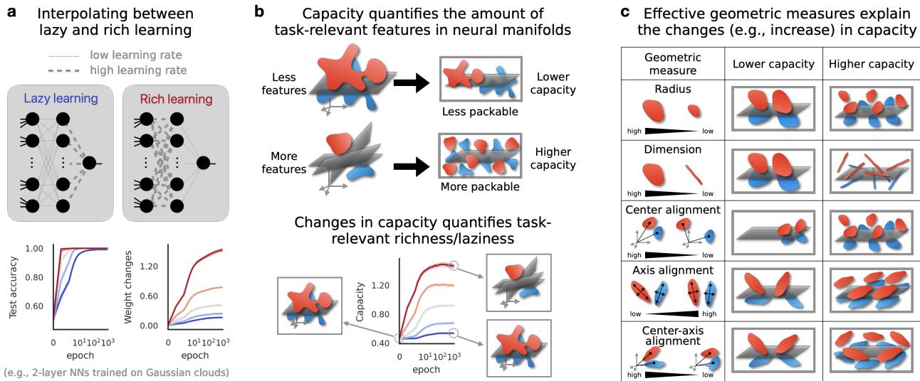
Part 2: Enter Manifold Capacity Theory

The authors propose shifting our focus from individual neurons or weights to Neural Manifolds.

What is a Neural Manifold?

Imagine you are showing a network pictures of dogs. Every picture of a dog creates a unique pattern of activity across the neurons in a layer. If you plot these patterns as points in a high-dimensional space (where each axis is a neuron), the collection of all “dog” points forms a cloud. This cloud is the Class Manifold.

If the network is doing a good job, the “dog” manifold should be distinct from the “cat” manifold. This process is called Manifold Untangling.

Measuring Untangling with Capacity

How do we quantify how well-separated these clouds are? The researchers utilize a concept called Manifold Capacity.

Think of the neural representation space as a physical container. Manifold Capacity measures how many distinct object manifolds you can pack into this container while still being able to separate them with a linear plane (a linear classifier).

• Low Capacity: The manifolds are tangled up, large, or messy. You can’t fit many of them in the space without them overlapping.
• High Capacity: The manifolds are tight, compact, and well-separated. You can pack many distinct categories into the same neural space.

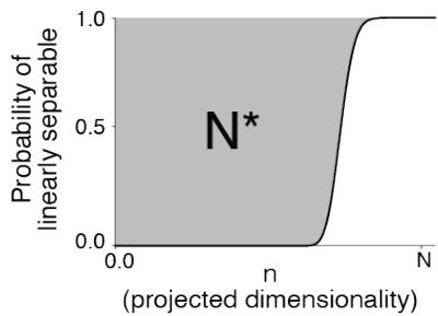
As shown in the figure above, capacity is related to the critical dimension required to separate the points. While the simulation definition is intuitive, it is computationally expensive to calculate for large networks.

The Mean-Field Solution

To make this practical, the authors use a “Mean-Field” theoretical definition (\(\alpha_M\)). This allows them to calculate capacity analytically using the geometry of the manifolds.

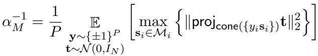
The crucial insight here is that Manifold Capacity (\(\alpha_M\)) is a direct proxy for the “Richness” of feature learning. As a network learns better features, it untangles the manifolds, and the capacity score goes up.

Part 3: GLUE (Geometry Linked to Untangling Efficiency)

Knowing that the capacity increased is useful, but knowing why it increased is profound. The authors introduce a set of geometric descriptors called GLUE.

The capacity of a set of manifolds is determined essentially by their size, shape, and orientation. The authors derived an approximation that links capacity (\(\alpha_M\)) to two primary geometric properties: Manifold Radius (\(R_M\)) and Manifold Dimension (\(D_M\)).

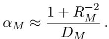
This equation is the “E=mc²” of representational geometry. It tells us two ways a neural network can improve its representation (increase \(\alpha_M\)):

1. Shrink the Radius (\(R_M\)): Make the point clouds smaller and tighter. This reduces the noise-to-signal ratio.
2. Compress the Dimension (\(D_M\)): Flatten the point clouds so they occupy fewer dimensions in the feature space.

The Geometric Descriptors

Beyond Radius and Dimension, the framework also tracks correlations between manifolds:

• Center Alignment (\(\rho_M^c\)): Are the centers of the different class clouds clustered together?
• Axes Alignment (\(\rho_M^a\)): are the “shapes” of the clouds oriented in the same direction?

By tracking these metrics, we can describe the strategy the network uses to learn.

Part 4: Validating the Metric

Does this actually work better than just looking at weight changes?

The researchers set up an experiment using 2-layer neural networks trained on synthetic data. They utilized a “scale factor” (\(\alpha\)) to artificially force the network into Lazy or Rich regimes. A small \(\alpha\) restricts feature learning (Lazy), while a large \(\alpha\) encourages it (Rich).

They compared Manifold Capacity against conventional metrics like “Weight Changes” and “Kernel Alignment” (CKA).

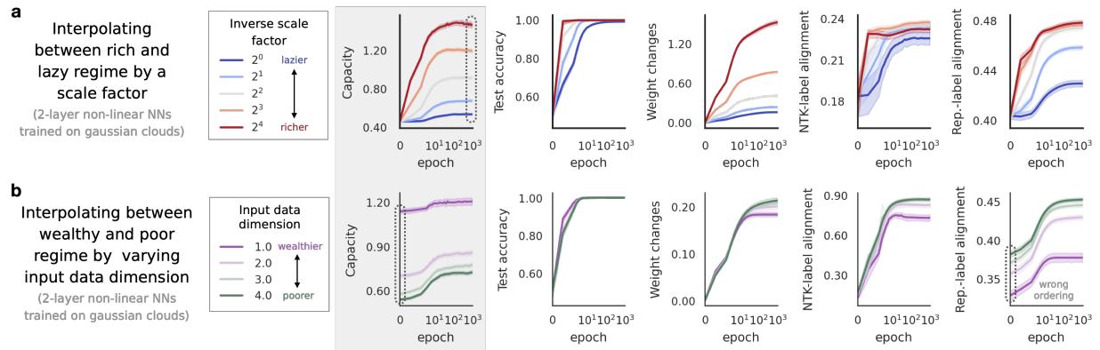
As seen in Figure 4a above:

• Test Accuracy saturates quickly; it can’t tell the difference between “somewhat rich” and “very rich.”
• Weight Changes explode in the rich regime but lack nuance.
• Capacity (the top row) shows a smooth, monotonic increase that perfectly tracks the ground-truth richness of the learning process.

It is not just an empirical observation; the authors provide a theoretical proof (Theorem 3.1) for 2-layer networks, showing that capacity mathematically tracks the effective degree of richness after a gradient step.

Part 5: Revealing Hidden Learning Dynamics

This is where the framework shines. Because Manifold Capacity is composed of geometric sub-components (Radius, Dimension, Alignment), we can decompose the learning process to see how the network is solving the problem.

Learning Strategies: Compression vs. Flattening

The authors discovered that networks don’t always learn the same way. By plotting the trajectory of learning on a Radius vs. Dimension plane, they identified distinct strategies.

• Strategy 1: Compress the radius first, then reduce dimension.
• Strategy 2: Sacrifice radius (let the manifolds expand slightly) to aggressively reduce dimensionality.

Learning Stages

Perhaps the most fascinating finding is that feature learning happens in distinct stages, even when the accuracy curve looks like a smooth line.

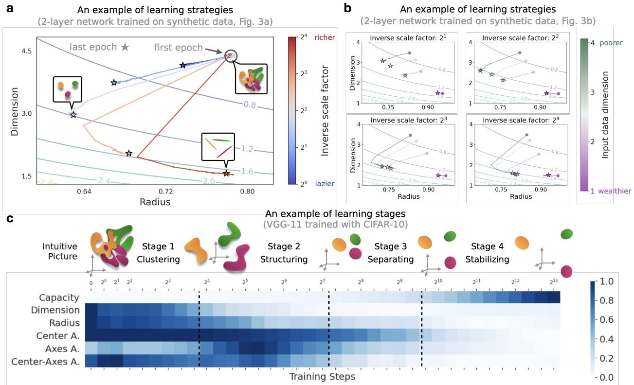
Looking at Figure 5c (above), we can identify four distinct phases in a deep network (VGG-11) training on CIFAR-10:

1. Clustering Stage: The network rapidly brings class manifolds together.
2. Structuring Stage: The geometric correlations (alignments) increase as the network figures out the relationships between classes.
3. Separating Stage: The alignments drop as the network pushes the distinct classes apart to maximize margin.
4. Stabilizing Stage: The geometry settles into its final configuration.

Standard accuracy metrics completely miss this drama happening beneath the surface.

Part 6: Applications in Neuroscience and ML

The power of this framework extends beyond analyzing toy models. The authors applied it to two major open problems.

1. Structural Bias in Recurrent Neural Networks (Neuroscience)

In neuroscience, it is difficult to measure synaptic weights directly. We can often only record neural activity. This makes “weight-based” analyses impossible.

The authors analyzed Recurrent Neural Networks (RNNs) trained on cognitive tasks. Previous work suggested that the initialization of the connectivity (specifically the rank of the weight matrix) biases the network toward lazy or rich learning.

Using Manifold Capacity, they found a nuanced result:

• RNNs with different initializations actually reach the same final capacity.
• However, they arrive there via totally different geometric paths. Low-rank initializations rely on changing dimensions, while high-rank initializations rely on changing radius.

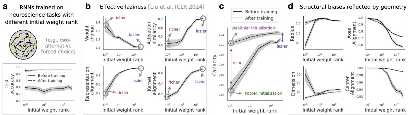
This suggests that the “structural inductive bias” of a brain circuit determines how it learns, even if the final performance is similar.

2. Out-of-Distribution (OOD) Generalization (Machine Learning)

A major plague in Deep Learning is OOD failure: a model works great on training data (e.g., CIFAR-10) but fails on slightly different data (e.g., CIFAR-100 or corrupted images).

Conventional wisdom might suggest that “Richer is always better.” If the network learns more features, shouldn’t it generalize better?

The authors found a counter-intuitive result: The “Ultra-Rich” regime hurts OOD generalization.

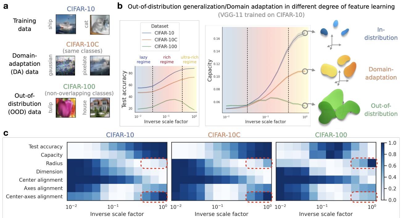
As shown in Figure 7, when the network is pushed into an “Ultra-Rich” regime (far right of the x-axis):

1. In-distribution accuracy (CIFAR-10) stays high.
2. OOD accuracy (CIFAR-100) crashes.

Why? The geometric analysis gives the answer: In the ultra-rich regime, the Manifold Radius expands and the Center-Axis Alignment increases. The network over-optimizes for the training data, creating “puffy,” highly aligned manifolds that are linearly separable for the specific training classes but structurally fragile when presented with new categories.

Conclusion

The dichotomy of “Lazy vs. Rich” has served the community well as a first-order approximation, but it is no longer enough. As this paper demonstrates, feature learning is a complex geometric process involving the compression, structuring, and untangling of high-dimensional manifolds.

By using Manifold Capacity and the GLUE metrics, we gain a diagnostic toolset that is:

1. Representation-based: It works on activations, not just weights.
2. Data-driven: It requires no assumptions about the data distribution.
3. Mechanistic: It explains why performance improves or degrades.

This geometric perspective opens new doors. For neuroscientists, it allows the analysis of brain plasticity using only activity recordings. For ML practitioners, it offers a new way to detect overfitting and predict OOD failure before deployment—simply by looking at the shape of the data clouds.

Feature learning is not just about moving weights; it’s about geometry. And now, we have the ruler to measure it.