Have you ever wondered why the first layer of almost every Convolutional Neural Network (CNN) looks the same? Whether you train a network to classify dogs, recognize cars, or detect tumors, the filters in the very first layer almost invariably converge to specific patterns: oriented edges and oscillating textures known as Gabor filters.

This phenomenon is one of the most robust empirical facts in deep learning. It mirrors the biology of the mammalian visual cortex, which also processes visual information using similar edge detectors. But why does this happen? And more importantly, what are the mathematical mechanics driving the learning of these features from raw pixels?

A recent research paper titled “Feature learning from non-Gaussian inputs: the case of Independent Component Analysis in high dimensions” tackles this question by connecting deep learning to a classic algorithm: Independent Component Analysis (ICA).

In this post, we will dive deep into this paper. We will explore why ICA is a perfect playground for understanding feature learning, why standard algorithms struggle in high dimensions, and how “smoothing” the loss landscape can drastically reduce the amount of data needed to learn.

The Mystery of the First Layer

Let’s start with the visual evidence. When we train a deep network like AlexNet on a massive dataset of natural images (like ImageNet), the weights adapt to extract useful features.

As shown in Figure 1 above:

• Panel (a) shows the filters learned by the first layer of AlexNet. They are localized, oriented, and resemble Gabor filters.
• Panel (b) shows filters learned by ICA on image patches. Notice the striking similarity? ICA also learns Gabor-like filters.
• Panel (c) shows filters learned by Principal Component Analysis (PCA). These look completely different—they are global, checkerboard-like patterns that don’t capture edges well.

This similarity between Deep Learning (DL) and ICA suggests that they are driven by the same underlying principle: Non-Gaussianity.

Natural images are highly non-Gaussian. Sky, grass, and skin textures don’t follow a simple bell curve distribution. ICA is designed specifically to hunt for these non-Gaussian directions. The researchers posit that ICA can serve as a “simplified, yet principled model” to study how deep networks learn features.

What is Independent Component Analysis (ICA)?

To understand the paper’s findings, we first need to define what ICA actually does.

Imagine you are at a cocktail party. You have two microphones recording the room. You hear a mix of two people talking simultaneously. ICA is the algorithm that can separate these mixed signals back into two independent voices.

Mathematically, ICA assumes the data is a linear mix of independent, non-Gaussian sources. The goal is to find a projection direction, defined by a weight vector \(w\), that makes the projected data as “non-Gaussian” as possible.

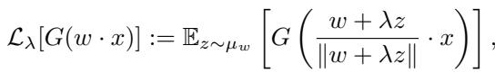
The objective function for ICA looks like this:

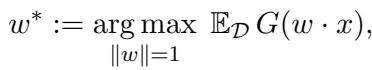
Here, \(w^*\) is the optimal direction we want to find, and \(G\) is a contrast function that measures non-Gaussianity. If the data were Gaussian, this function wouldn’t help us find interesting directions (since a Gaussian looks the same from all angles). But since our “signal” is non-Gaussian, maximizing \(G(w \cdot x)\) points us toward the feature.

Common choices for the contrast function \(G(s)\) include:

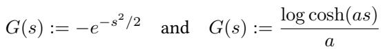
The first choice (negative exponential) is robust to outliers, while the second is related to kurtosis (the “tailedness” of a distribution).

The High-Dimensional Problem

Here is where the paper shifts from observation to rigorous analysis. In modern machine learning, we deal with high-dimensional data (\(d\) is large). A \(64 \times 64\) image patch has 4,096 dimensions.

Classic theories about ICA focus on asymptotic convergence (what happens when we have infinite time). But in high dimensions, the main bottleneck isn’t convergence speed—it’s the search phase. The algorithm starts with random weights. In a massive 4000-dimensional space, how many samples (\(n\)) does the algorithm need to even find the right direction and escape the randomness?

The authors investigate two main algorithms:

1. FastICA: The standard, industry-standard algorithm for ICA.
2. Stochastic Gradient Descent (SGD): The algorithm used to train neural networks.

The Synthetic Setup: The Spiked Cumulant Model

To measure performance precisely, the authors use a controlled synthetic data model called the Spiked Cumulant Model.

Imagine a dataset where the data looks like standard Gaussian noise in every direction except one. In that one special direction (the “spike” or signal \(v\)), the data follows a non-Gaussian distribution.

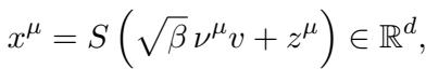
Here:

• \(x^\mu\) is the input vector.
• \(v\) is the hidden non-Gaussian direction (the feature we want to learn).
• \(\nu^\mu\) is the latent non-Gaussian signal (e.g., random \(\pm 1\) values).
• \(z^\mu\) is Gaussian noise.
• \(S\) is a whitening matrix (which ensures we can’t cheat by using simple variance/PCA methods).

The whitening matrix is defined as:

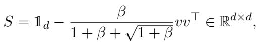
This setup creates a “needle in a haystack” problem. The algorithm must process \(n\) samples to find the vector \(v\) hidden inside a \(d\)-dimensional space.

Result 1: FastICA requires a Massive Amount of Data

FastICA is a fixed-point algorithm. It updates its estimate of the weights \(w\) using the entire dataset at once (large batch). The update rule looks like this:

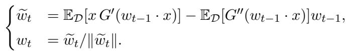
It has two parts: a gradient-like term and a regularization term. This regularization is famous for making FastICA converge very quickly (quadratically) once it is close to the solution.

But does it find the solution from a random start?

The authors prove a startling result. For the FastICA algorithm to recover a single non-Gaussian direction in high dimensions, the number of samples \(n\) must scale with the fourth power of the dimension \(d\).

In the world of high-dimensional statistics, \(d^4\) is a disaster. If your input dimension is just 100, you would need \(100^4 = 100,000,000\) samples.

The researchers confirmed this theoretical bound with experiments. Look closely at Figure 2:

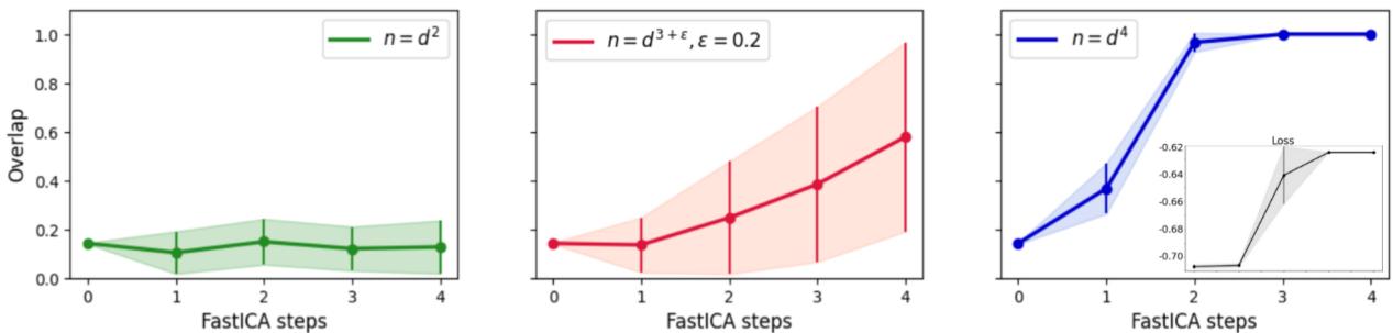
• Left Graph (\(n = d^2\)): The algorithm fails. The overlap (similarity between learned weight and true feature) stays low, near the random baseline.
• Middle Graph (\(n = d^{3.2}\)): It’s struggling, slowly climbing but unstable.
• Right Graph (\(n = d^4\)): Success! The overlap jumps to nearly 1.0 (perfect recovery) very quickly.

This confirms the theory: FastICA is incredibly data-inefficient for the search phase in high dimensions.

Why is it so hard? The Information Exponent

Why does it take \(d^4\) samples? The mathematical explanation involves the Information Exponent (\(k^*\)).

The population loss function can be expanded into a series of terms based on the overlap \(\alpha\) between our weights and the true signal.

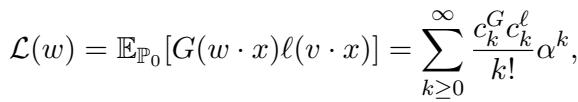
Because the data is whitened (covariance is identity), the first few terms of this expansion vanish. The first non-zero term for this specific ICA problem appears at the fourth order (\(k^* = 4\)).

Roughly speaking, the “signal” strength scales like \(\alpha^{k^*-1}\). At initialization, we are randomly guessing, so our overlap \(\alpha\) is tiny (\(\approx 1/\sqrt{d}\)). This makes the signal incredibly weak—scaling as \(d^{-3/2}\). The noise, meanwhile, scales with the sample size. To distinguish that tiny signal from the noise, you need a massive number of samples proportional to \(d^{k^*}\).

Result 2: SGD and Smoothing the Landscape

If FastICA requires \(d^4\) samples, is there a better way?

The authors turn to Stochastic Gradient Descent (SGD), the workhorse of deep learning. They analyze Online SGD, where you update weights one sample at a time.

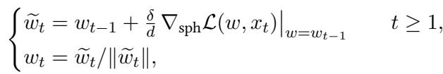
Theory from previous work suggests that standard Online SGD requires \(n \approx d^{k^*-1}\) samples. Since \(k^*=4\), vanilla SGD should work with \(n \approx d^3\) samples. This is better than FastICA (\(d^4\)), but still quite expensive.

However, the authors introduce a powerful modification: Smoothed SGD.

Smoothing the Loss

The problem with high-dimensional optimization is that the loss landscape is often very flat around the initialization point (a saddle point). The gradient is tiny and noisy, making it hard to see which way is “down.”

Smoothing involves convoluting the loss function with a Gaussian kernel. Instead of looking at the loss at exactly point \(w\), we look at the average loss in a small neighborhood around \(w\).

Here, \(\lambda\) controls the radius of the smoothing. A large \(\lambda\) means we look further afield.

Why does this help? Imagine you are hiking in a landscape with a very narrow, steep canyon (the minimum) hidden in a vast, flat plain. If you stand on the plain, you see no slope. But if you “smooth” the landscape, the influence of the deep canyon spreads out, creating a gentle slope on the plain that points you toward the canyon.

Visually, smoothing changes the shape of the loss function near zero (where we start):

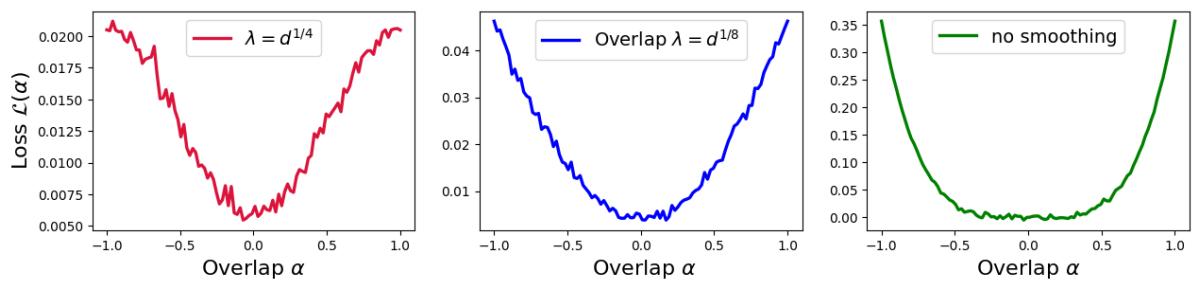
• The green line (No smoothing) is flat at the bottom. It’s hard to find a gradient.
• The red line (Large smoothing \(\lambda = d^{1/4}\)) is sharper and V-shaped. It provides a stronger gradient signal even when we are far from the solution.

Closing the Gap

The authors prove that by carefully choosing the smoothing parameter \(\lambda\), they can reduce the sample complexity of SGD from \(d^3\) down to \(d^2\).

This \(n \approx d^2\) threshold is significant because it represents the computational limit for polynomial-time algorithms in this setting.

The experiment in Figure 3 confirms this hierarchy:

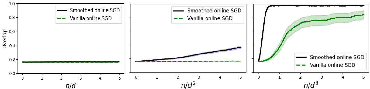
• Left (\(n \propto d\)): Neither algorithm works.
• Middle (\(n \propto d^2\)): Smoothed SGD (black line) recovers the signal! Vanilla SGD (green dashed) fails.
• Right (\(n \propto d^3\)): Now both algorithms work.

This demonstrates that smoothing effectively “boosts” the signal, allowing the network to learn features with significantly less data.

Back to Reality: FastICA on ImageNet

We have established that on synthetic data, FastICA is inefficient (\(d^4\)) and Smoothed SGD is optimal (\(d^2\)). But wait—didn’t we see in the introduction that FastICA works well on real images?

The authors returned to the ImageNet dataset to test FastICA’s actual performance.

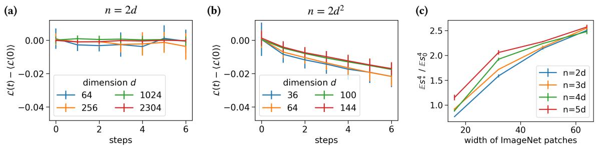
In Figure 4:

• Panel (a): With linear samples (\(n=2d\)), FastICA is stuck.
• Panel (b): With quadratic samples (\(n=2d^2\)), FastICA succeeds in lowering the loss.

Wait, didn’t we just prove FastICA needs \(d^4\) samples? Why is it working at \(d^2\) on real images?

The answer lies in the Signal-to-Noise Ratio (SNR) of real data. The synthetic “Spiked Cumulant Model” assumes the hidden signal is somewhat subtle (a specific statistical property). However, natural images are extremely non-Gaussian. They have heavy tails and strong kurtosis.

The authors measured the “strength” of the non-Gaussian signal in ImageNet (Panel c) and found it to be much higher than in the synthetic models. This massive inherent signal in real images compensates for FastICA’s inefficiency. The “spike” in real data is so huge that even a suboptimal algorithm can find it quickly.

Conclusion: Implications for Deep Learning

This paper takes us on a journey from the visual similarity of CNN filters to the hard mathematical limits of feature learning.

Here are the key takeaways:

1. ICA is a valid model for Feature Learning: It explains the emergence of Gabor filters solely through the maximization of non-Gaussianity.
2. FastICA has a “Search Phase” problem: In high dimensions, standard algorithms can get stuck blindly searching for a signal, theoretically requiring \(n \approx d^4\) samples.
3. Smoothing is powerful: By smoothing the loss landscape, we can accelerate SGD to learn with optimal sample efficiency (\(n \approx d^2\)). This mimics how neural networks (which often inherently smooth their inputs or gradients) might operate.
4. Real Data is Forgiving: The strong non-Gaussian structure of natural images makes feature learning easier than worst-case theoretical bounds suggest.

Understanding these dynamics helps explain why deep learning works so well on images and suggests that techniques like loss smoothing could be vital for domains where the data isn’t as “loud” as ImageNet.