](https://deep-paper.org/en/paper/2504.05806/images/cover.png)
Neural Fields are one of the most exciting developments in machine learning today. You’ve likely seen their most famous application—Neural Radiance Fields (NeRFs)—which can generate stunning, photorealistic 3D scenes from just a handful of 2D images. At their core, Neural Fields (NFs) are simple but powerful: they use a neural network to map input coordinates (like \((x, y)\) for an image or \((x, y, z)\) for a 3D scene) to an output value (such as RGB color or density). This elegant approach enables continuous data representation across modalities—images, audio, video, or 3D spaces—with impressive compactness.
Yet, this approach faces two major challenges.
- Training speed: fitting a neural field from scratch for a single scene can take hours or even days.
- Catastrophic forgetting: when retrained on new data, neural networks often overwrite previous knowledge.
Imagine a drone mapping a city block by block, or a satellite capturing the same region over time. The model must learn sequentially, without forgetting past information, and adapt rapidly to new data.
A recent paper from Seoul National University— “Meta-Continual Learning of Neural Fields (MCL-NF)” —tackles this challenge head-on. It introduces a new problem setting and a framework that unites the adaptability of meta-learning with the stability of continual learning. Let’s unpack how it works.
Understanding the Foundations
To grasp MCL-NF’s innovation, let’s revisit three fundamental pillars: Neural Fields (NF), Continual Learning (CL), and Meta-Learning (ML).
Neural Fields (NF)
A neural field is a function, parameterized by a neural network \(f_{\theta}\), that maps a coordinate \(x\) to a value \(y\).
- For a 2D image: \(x = (x, y)\) → \(y = (R, G, B)\).
- For a 3D NeRF: \(x = (x, y, z, \theta, \phi)\) → \(y = (\text{color}, \text{density})\).
All scene information is encoded in the parameters \(\theta\), making NFs memory-efficient yet slow to train.
Continual Learning (CL)
Continual Learning deals with training a model on a sequence of tasks \(\mathcal{T}_1, \mathcal{T}_2, \ldots, \mathcal{T}_n\), where past data isn’t always accessible. The goal is to acquire new knowledge while retaining previous learning.
Common CL strategies:
- Replay-based methods: store and revisit past samples while training new ones.
- Regularization-based methods: restrict changes to parameters crucial for older tasks.
- Modular approaches: assign different parts (modules) of the network to separate tasks, preventing interference.
Meta-Learning (ML)
Meta-learning, or “learning to learn,” focuses on rapid adaptation. The most widely used algorithm, Model-Agnostic Meta-Learning (MAML), learns an effective initialization—\(\theta_0\)—so that new tasks can converge quickly after a few gradient updates. MAML doesn’t aim to prevent forgetting; it optimizes for fast learning.
MCL-NF attempts to integrate the speed of ML and the memory retention of CL, crafting a model that learns fast and remembers well.
The Core Innovation: Three Pillars of MCL-NF
The MCL-NF framework combines (1) modularization with shared initialization, (2) a novel Fisher Information-based loss, and (3) theoretical guarantees for stability and convergence.
1. Modularization with Shared Meta-Learned Initialization
The architecture is modular: rather than one monolithic network, each task is assigned to its own module. Consider the examples:
- In a video: each frame or group of frames becomes a task-specific module.
- In a large-scale NeRF: each city block is modeled as an independent module.
This structure prevents catastrophic forgetting by keeping parameters distinct per task. However, the key insight lies in shared initialization via MAML.
During meta-training, the system learns a universal initialization \(\theta_{\text{shared}}\). During meta-testing, each new module begins from \(\theta_{\text{shared}}\) and fine-tunes itself to its unique task.
This setup combines:
- Isolation (modules remember their own tasks).
- Speed (all modules start from an optimized initialization).
The result is rapid convergence and persistent memory.
2. FIM-Loss: Prioritizing Informative Samples
Even modular models can be redundant. For example, two adjacent city blocks may share overlapping visual patterns. To learn efficiently, the model should focus on informative samples that contribute most to parameter improvement.
The second innovation introduces the Fisher Information Maximization Loss (FIM-Loss)—a reweighted version of the standard Mean Squared Error (MSE).
Standard MAML minimizes an MSE-based objective:
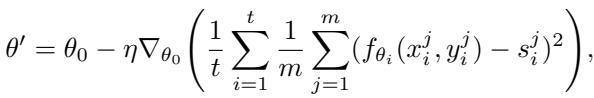
Figure: Standard MAML objective function minimizes MSE across tasks.
The authors modify this by introducing a sample-specific weight \(w_{ij}\):
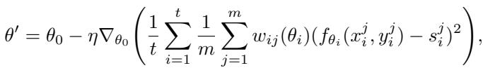
Figure: FIM-Loss incorporates sample-specific weights derived from Fisher Information.
The weight \(w_{ij}\) is computed using the Fisher Information Matrix (FIM), which quantifies how much information a data sample contributes to refining a model’s parameters:
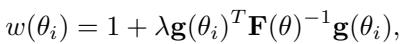
Figure: Weight term depends on a hyperparameter \( \lambda \), the gradient vector \( \mathbf{g} \), and the inverse Fisher Information Matrix.
Here’s how it works:
- \(\mathbf{g}(\theta_i)\): gradient of log-likelihood for the sample—represents sensitivity or “surprise.”
- \(\mathbf{F}(\theta)^{-1}\): inverse Fisher matrix—normalizes parameter importance.
- \(\lambda\): controls the influence of Fisher Information.
By amplifying losses from high-information samples, the model “studies harder” where it matters most—achieving faster learning and better generalization.
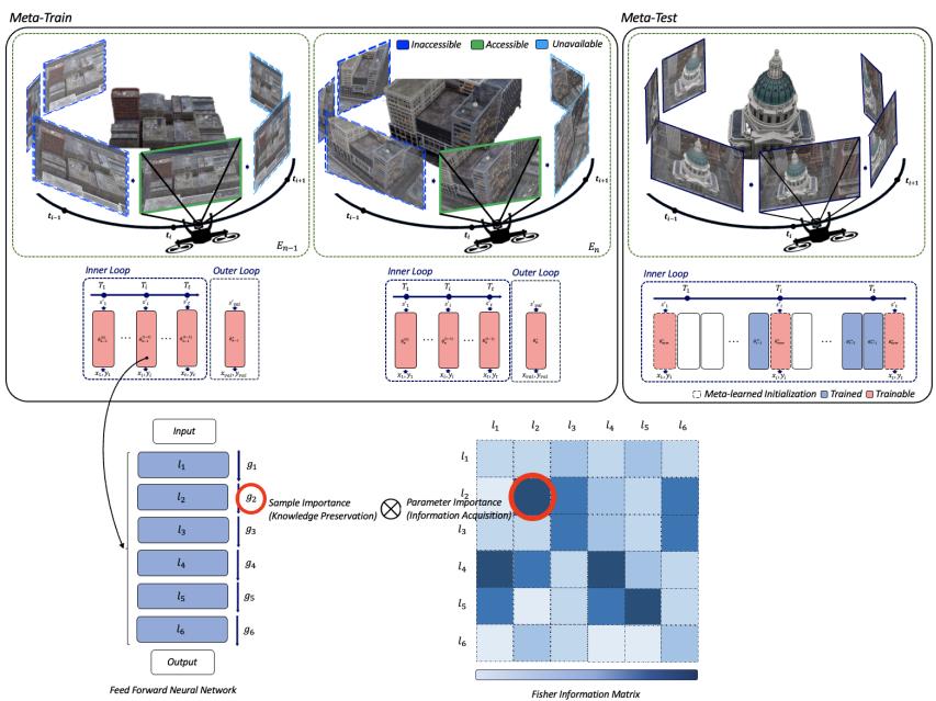
Figure: Transition from traditional MSE loss to FIM-Loss shows how sample weights guide learning toward informative regions.
Unlike previous Fisher-based approaches like Elastic Weight Consolidation (EWC)—which use Fisher Information at the parameter level to maintain old knowledge—FIM-Loss operates at the sample level, dynamically improving efficiency and adaptability.
3. Theoretical Guarantees
To ground their approach mathematically, the authors show that FIM-Loss is connected to information gain maximization.
They prove that the Fisher Information gives a local approximation of KL-divergence between parameter distributions:
\[ KL[p(\mathcal{D}|\theta)||p(\mathcal{D}|\theta + \Delta\theta)] \approx \frac{1}{2} \Delta \theta^{T} \mathbf{F}(\theta) \Delta \theta \]This demonstrates that optimizing with FIM implicitly maximizes mutual information between parameters and data—boosting generalization while ensuring stable convergence. Their theoretical analysis also provides convergence and generalization bounds for FIM-augmented Stochastic Gradient Descent (FIM-SGD), confirming that MCL-NF isn’t just practical but provably reliable.
Experiments: Learning Across Modalities
The researchers tested MCL-NF across a diverse range of tasks and datasets:
- Image Reconstruction: CelebA, FFHQ, ImageNette
- Video Reconstruction: VoxCeleb2
- Audio Reconstruction: LibriSpeech
- View Synthesis (NeRF): MatrixCity
They compared their methods— “Ours (mod)” (modular) and “Ours (MIM)” (modular + FIM-Loss)—against baselines such as ER, EWC, MAML+CL, and OML.
Rapid Adaptation and High Fidelity
Reconstruction quality was measured using PSNR (higher is better) against the number of test-time optimization steps.
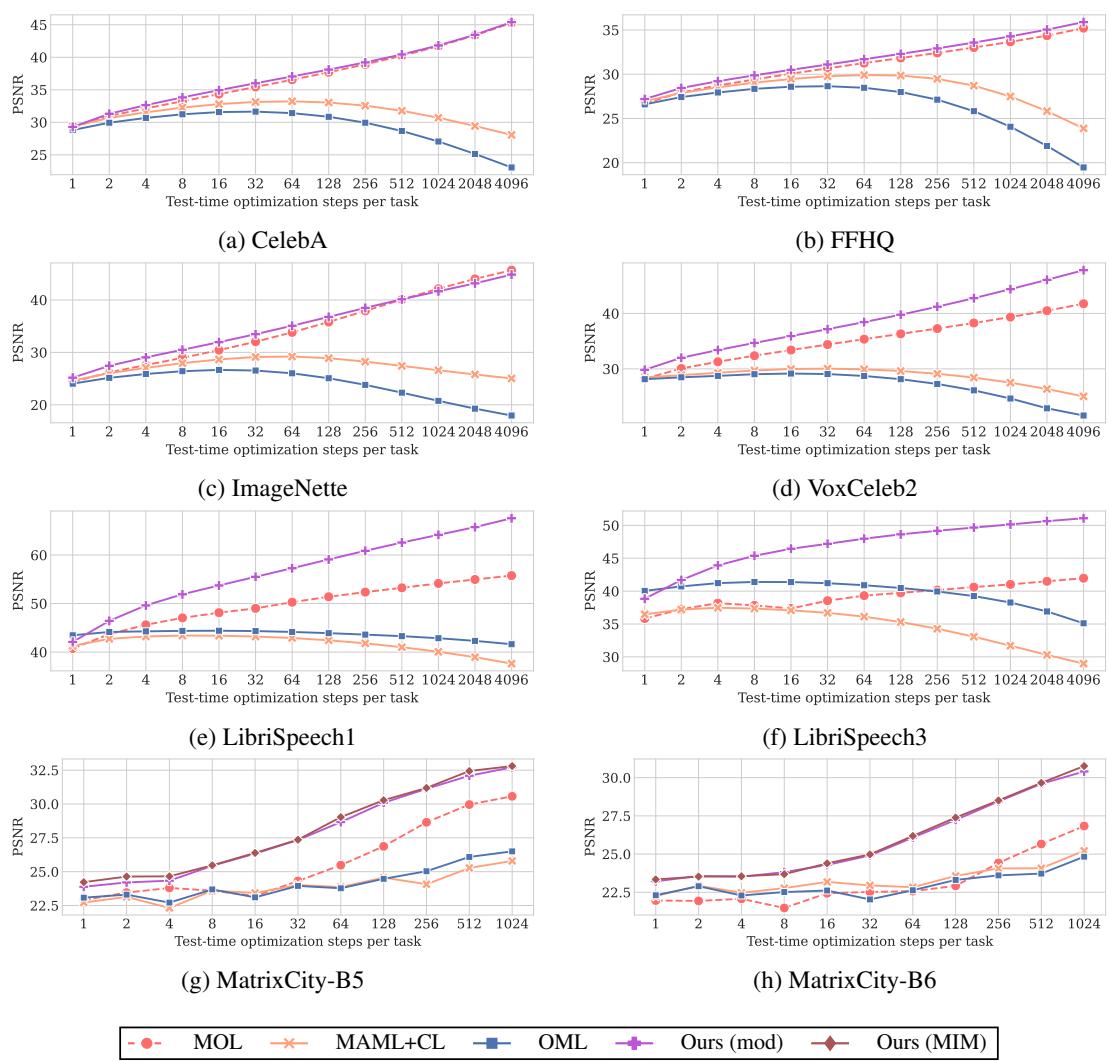
Figure 2: PSNR comparison over adaptation steps. MCL-NF shows consistent improvement and superior final quality.
Across all datasets, the proposed methods achieved higher PSNR with fewer steps. While MAML+CL and OML plateau early, MCL-NF continues stable improvement, demonstrating both fast convergence and long-term stability—addressing catastrophic forgetting effectively.
Quantitative Strength at Scale
Performance comparisons across modalities confirm the superiority of MCL-NF.
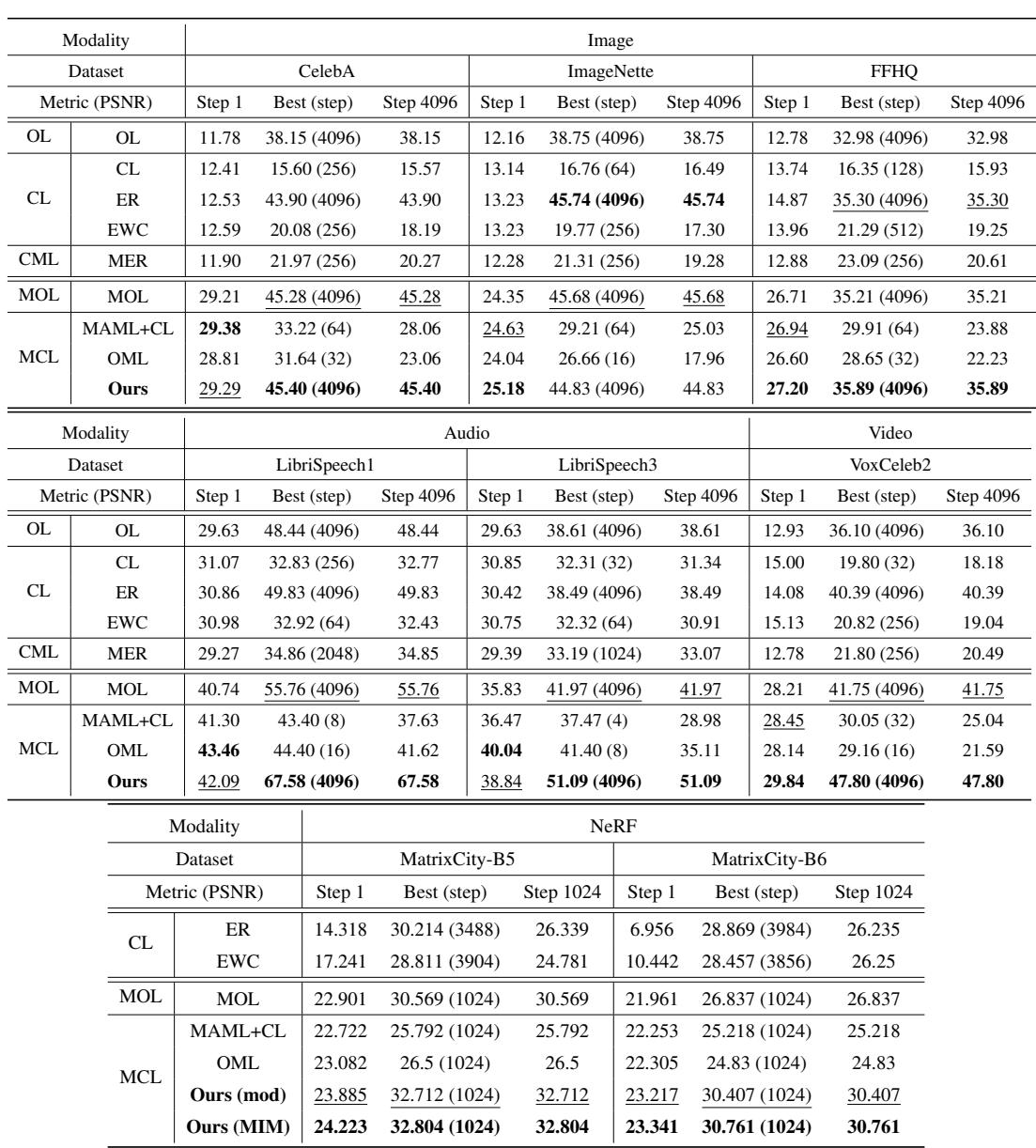
Figure 3: Quantitative results across all methods and datasets. MCL-NF achieves top or near-top performance throughout training.
Whether evaluated at Step 1, peak step, or final step 4096, MCL-NF consistently ranks first or second—showing both strong initialization and sustained progress.
Visual Quality: Seeing the Difference
The qualitative results highlight real-world visual improvements.
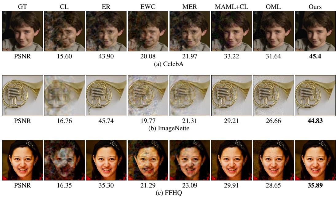
Figure 4: Visual comparisons across CelebA, FFHQ, and ImageNette. “Ours” consistently produces sharper, cleaner reconstructions.
Images generated by MCL-NF are noticeably clearer and artifact-free compared to baseline methods, showing accurate color reproduction and fine-grained detail preservation.
Scaling Up: City-Sized Neural Fields
The most impressive showcase is MatrixCity, a benchmark for city-scale view synthesis. Training a NeRF for an entire city usually requires enormous resources. By partitioning the city into modules (tasks) and employing shared initialization, MCL-NF efficiently manages this large-scale rendering while maintaining high fidelity at reduced parameter counts.
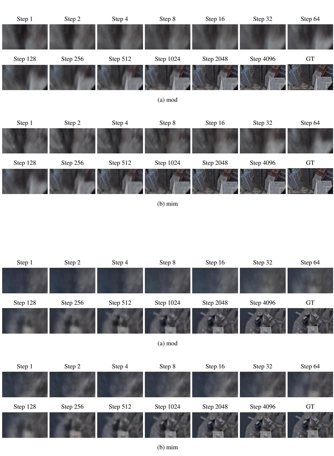
Figure 5: Reconstruction progression in city-scale NeRF rendering. “MIM” shows faster and sharper refinement through optimization steps.
Successive visualizations show progressive sharpening of details with each optimization step, ultimately producing crisp, realistic cityscapes—an indicator of strong scalability and robustness even in complex environments.
Conclusions and Outlook
The Meta-Continual Learning of Neural Fields (MCL-NF) framework delivers a unified solution for continual, rapid learning in resource-constrained scenarios. By combining:
- modular architectures for memory stability,
- meta-learned shared initialization for fast adaptation, and
- information-theoretic FIM-Loss for intelligent sample weighting,
MCL-NF overcomes catastrophic forgetting and achieves exceptional learning efficiency across images, audio, video, and 3D rendering tasks.
This work paves the way for adaptive systems that can learn on the fly—ideal for drones, autonomous navigation, environmental monitoring, and real-time city-scale modeling. While challenges remain, such as potential memory overhead with increasing modules, the study marks a significant stride toward truly continual, scalable neural field learning.
In short, MCL-NF represents a compelling step forward in bridging the gap between speed and stability—helping neural fields continue to learn, remember, and evolve as fluidly as the dynamic worlds they aim to model.