Introduction

In the world of high-dimensional statistics and machine learning, few problems are as classic or as stubborn as learning Gaussian Mixture Models (GMMs). We use them everywhere—from astrophysics to marketing—to model populations made up of different sub-groups.

The theoretical landscape of GMMs is a tale of two extremes. On one hand, if the components are spherical (perfectly round blobs), we can learn them efficiently. On the other hand, if the components are arbitrary “pancakes” (highly flattened Gaussians) that are stacked parallel to each other, the problem becomes exponentially hard. In the worst case, learning a mixture of \(k\) Gaussians in \(d\) dimensions requires time \(d^{O(k)}\).

Recent research has tried to find a middle ground. What if we assume the mixing weights (the proportion of the population belonging to each component) aren’t vanishingly small? Algorithms were found that run in quasi-polynomial time, specifically \(d^{O(\log(1/w_{\min}))}\).

This brings us to a fascinating new paper: “On Learning Parallel Pancakes with Mostly Uniform Weights.”

This research tackles two fundamental questions:

1. Is the current quasi-polynomial speed limit real? Can we do better if the weights are perfectly uniform (\(1/k\))?
2. What if the weights are “mostly” uniform? What if most components are balanced, but a few outlier components have arbitrary weights?

In this post, we will dive deep into this paper. We will explore why “Parallel Pancakes” are so hard to detect, proving that even with uniform weights, we hit a computational wall. Then, we will look at a clever new algorithmic result showing that if the weights are mostly equal, the problem becomes much easier.

Background: The Problem with Pancakes

To understand the contribution of this paper, we first need to define the “Parallel Pancakes” problem.

Imagine you have a distribution of data in high-dimensional space (\(d\) dimensions).

• The Null Hypothesis (\(H_0\)): The data is just standard Gaussian noise, \(\mathcal{N}(0, I)\). It looks like a fuzzy hypersphere centered at the origin.
• The Alternative Hypothesis (\(H_1\)): The data comes from a mixture of \(k\) Gaussians. However, these aren’t just any Gaussians. Their means are all lined up along a single unknown direction \(v\), and they are flattened (squashed) along that same direction. In all orthogonal directions, they look like standard Gaussians.

Because they are flattened and stacked along one line, they resemble a stack of pancakes floating in high-dimensional space.

The challenge is to distinguish between these two cases. This is known as the Non-Gaussian Component Analysis (NGCA) problem. If the pancakes are stacked just right, their combined density along the direction \(v\) can mimic a standard Gaussian almost perfectly. If the mixture matches the first \(m\) moments of a standard Gaussian, identifying the hidden direction \(v\) requires roughly \(d^{m}\) samples or queries.

The SQ Model

The authors analyze this problem using the Statistical Query (SQ) model. Instead of looking at individual data points, an SQ algorithm asks questions like: “What is the expected value of this function \(f(x)\) over the distribution?” The oracle returns the answer with some tolerance \(\tau\).

This model is powerful because it covers almost all standard techniques (SGD, spectral methods, moment matching). Proving a lower bound in the SQ model is a strong indicator that the problem is computationally hard for any noise-tolerant algorithm.

Part 1: The Bad News (SQ Lower Bounds)

The first major contribution of the paper is a lower bound. Previous algorithms achieved a complexity of \(d^{O(\log k)}\) for mixtures where the minimum weight \(w_{\min}\) is polynomial in \(k\). The authors asked: If we make the problem “easier” by enforcing that all weights are exactly equal (\(w_i = 1/k\)), can we get a polynomial time algorithm?

The answer is no.

Theorem 1.2 in the paper states that even with uniform weights, any SQ algorithm requires \(d^{\Omega(\log k)}\) complexity. This proves that the existing quasi-polynomial algorithms are essentially optimal.

The Strategy: Moment Matching Designs

To prove this hardness, the authors construct a “bad” distribution. They need to find a set of \(k\) points in 1D space (representing the centers of the pancakes) such that the uniform distribution over these points matches the first \(m = \Omega(\log k)\) moments of a standard Gaussian.

If such a distribution exists, they can create a Parallel Pancake instance that “looks” like a standard Gaussian up to moment \(m\). Standard SQ results tell us that distinguishing this mixture takes \(d^{\Omega(m)}\) time.

The proof relies on design theory. Specifically, they need to show the existence of a discrete distribution supported on an interval that matches moments with the Gaussian.

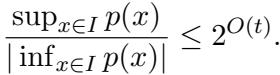
The crucial metric here is \(K_t\), a value that bounds the ratio of the maximum to the minimum magnitude of a polynomial on an interval. If this ratio is bounded by \(2^{O(t)}\), a design of size \(t\) exists.

To bound this ratio, the authors use properties of Hermite polynomials. They expand an arbitrary polynomial \(p(x)\) in the Hermite basis.

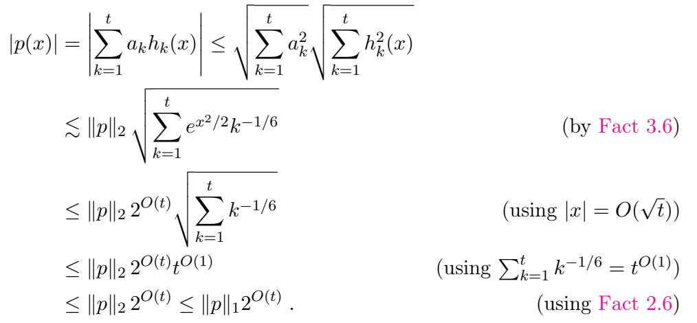
By using the fact that Hermite polynomials are bounded (weighted by the Gaussian density) and applying anti-concentration inequalities, they show that a polynomial cannot stay “too small” over the interval relative to its norm.

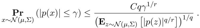
Specifically, they use the Carbery-Wright inequality to ensure the polynomial isn’t “flat” near zero:

By combining these bounds, they prove that you can indeed stack \(k\) uniform pancakes in a way that matches \(\log k\) moments of a standard Gaussian. Therefore, the problem remains quasi-polynomial hard.

Part 2: The Good News (Mostly Uniform Weights)

While the uniform case is hard, the second contribution of the paper offers a new perspective. The previous best algorithms had complexity depending on \(1/w_{\min}\). If even one component had a tiny weight (e.g., \(2^{-k}\)), the runtime would explode to exponential.

The authors propose a “mostly uniform” setting:

• \(k'\) components have arbitrary weights.
• The remaining \(k - k'\) components have equal weights.

Theorem 1.3 presents an algorithm that solves the testing problem with sample complexity roughly \((kd)^{O(k' + \log k)}\).

This is a significant improvement because it interpolates between the hard and easy regimes. If you have only a few “weird” weighted components, the complexity doesn’t blow up based on how small their weights are—it only depends on how many (\(k'\)) of them there are.

The Core Logic: Impossibility of Moment Matching

The algorithm works because of a key structural insight: A “mostly uniform” mixture cannot fake being a Gaussian for very long.

While a fully arbitrary mixture might match moments up to \(k\), and a fully uniform mixture up to \(\log k\), a mixture with only \(k'\) arbitrary weights can only match moments up to \(m \approx O(k' + \log k)\).

If the mixture fails to match the \((m+1)\)-th moment, the algorithm can detect it by simply estimating the moment tensors from data and comparing them to the standard Gaussian tensor.

The Proof: Bounding the Moments

How do they prove that matching more than \(O(k' + \log k)\) moments is impossible? This is the technical heart of the paper.

Let \(A\) be the discrete distribution of the pancake centers. Suppose \(A\) matches the first \(m\) moments of the standard Gaussian. We define a polynomial \(p(x)\) that vanishes (is zero) at the \(k'\) locations where the weights are arbitrary.

We then look at the function \(f(x) = x^t p(x)\). The goal is to derive a contradiction by looking at the ratio of expectations:

\[ \frac{\mathbb{E}_{x \sim A}[f^2(x)]}{(\mathbb{E}_{x \sim A}[f(x)])^2} \]

First, the authors derive an upper bound for this ratio. Because \(p(x)\) zeros out the arbitrary weights, the expectation depends only on the uniform weights. This leads to the inequality:

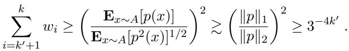
Essentially, because the weights are uniform (and roughly \(1/k\)), this ratio cannot be too large.

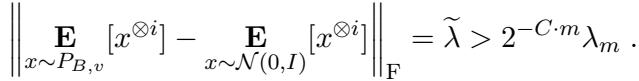
Next, they need a lower bound. They assume, for the sake of contradiction, that the distribution \(A\) matches the moments of the Gaussian \(\mathcal{N}(0,1)\). This allows them to replace expectations over \(A\) with expectations over the Gaussian (plus a tiny error term \(\lambda\)).

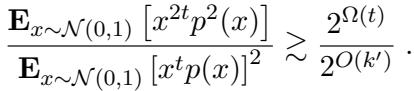
To get the contradiction, they need to show that the Left Hand Side (the ratio under the Gaussian measure) is actually very large—larger than the upper bound allowed by the uniform weights.

This requires proving that the polynomial \(x^{2t}p^2(x)\) has a large expectation relative to the square of the expectation of \(x^t p(x)\).

The Continuous AM-GM Trick

To prove the inequality in Figure 16 (above), the authors use a beautiful analytical technique involving the Arithmetic Mean-Geometric Mean (AM-GM) inequality for integrals.

They analyze the integral of the polynomial over a specific interval \(I = [0.9\sqrt{2t}, 1.1\sqrt{2t}]\). They need to lower bound the “energy” of the polynomial \(p(x)\) in this region.

Using the continuous AM-GM inequality, they relate the arithmetic mean of \(p^2(x)\) to the geometric mean, which involves the integral of \(\ln|p(x)|\):

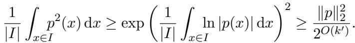
This transforms the problem into bounding the integral of a logarithm of a polynomial. Since \(p(x) = \prod (x - \mu_i)\), the log breaks down into a sum of logs:

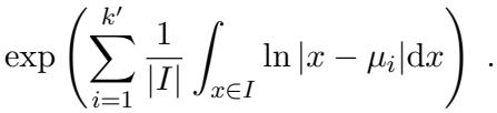
The authors then perform a detailed case analysis on the location of the roots \(\mu_i\) relative to the interval \(I\). By integrating \(\ln|x - \mu_i|\), they show that the “geometric mean” of the polynomial on this interval cannot be too small.

After summing these contributions and exponentiating, they arrive at a lower bound for the numerator of their ratio.

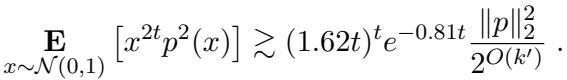
Combining this with an upper bound on the denominator (using standard Gaussian hypercontractivity), they force the ratio to be at least \(2^{\Omega(t)}\).

Since the upper bound derived from the weights was roughly \(k\), and the lower bound is exponential in \(t\), we get a limit on \(t\):

\[ t \lesssim \log k + k' \]

This proves that you cannot match more moments than this threshold!

The Algorithm

Armed with the knowledge that the moments must differ at some degree \(m \approx O(k' + \log k)\), the algorithm is straightforward (conceptually).

1. Calculate Tensor Gap: We know that for some \(i \leq m\), the difference between the \(i\)-th moment tensor of our data and the standard Gaussian tensor is significant.

2. Sample and Verify: The algorithm draws samples and computes the empirical tensor.

3. Thresholding: If the empirical tensor differs from the Gaussian tensor by more than a specific threshold (derived from the theoretical gap), we reject the Null Hypothesis and declare “Pancakes!”

There is one technical caveat: the sample complexity depends on the data being well-behaved (concentrated). To ensure this, the authors add a check to verify that no data points are absurdly far from the origin, which could mess up the tensor estimation.

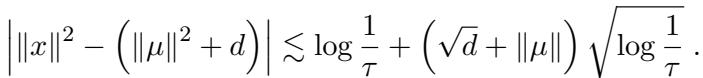
This ensures that the empirical averages converge quickly to the true expectations.

Conclusion

The paper “On Learning Parallel Pancakes with Mostly Uniform Weights” provides a tight resolution to the problem of learning GMMs with common covariance.

1. The Limitation: We now know that the quasi-polynomial time complexity for learning parallel pancakes isn’t just an artifact of our current algorithms—it’s baked into the geometry of the problem via SQ lower bounds. Even uniform weights don’t save us.
2. The Interpolation: However, the paper gives us a hopeful path forward for “messy” data. If we have a background of uniform noise/components sprinkled with a few arbitrary signals, we can detect them efficiently. The complexity scales with the number of arbitrary components (\(k'\)), not their weight.

This work beautifully combines combinatorics (design theory), analysis (polynomial approximation), and statistics (SQ model) to map out the boundaries of what is computationally learnable in high dimensions.

---

This blog post explains the research paper “On Learning Parallel Pancakes with Mostly Uniform Weights” by Diakonikolas et al. (2025).

---