Learning to See Without Looking—How AI Can Avoid Missing Data

If you have ever worked with real-world datasets, particularly in healthcare or finance, you know the pain of missing values. You design a perfect model, train it on cleaned data, and prepare it for deployment. But then comes “test time”—the moment your model faces a real user. The user skips a question on a form, or a specific medical test hasn’t been ordered yet. Suddenly, your model is blind in one eye.

How do we handle this? The standard playbook suggests two paths: imputation (guessing the missing value based on averages or patterns) or missingness indicators (adding a flag telling the model “this data is missing”).

While these methods work computationally, they introduce a hidden danger: reliability and interpretability. If a model predicts a high risk of heart disease because it guessed a missing blood pressure value, can a doctor trust it?

In the paper “Prediction Models That Learn to Avoid Missing Values,” researchers Stempfle, Matsson, Mwai, and Johansson propose a refreshing alternative. Instead of teaching models to guess what isn’t there, they teach models to avoid needing the missing data in the first place.

This approach, called Missingness-Avoiding (MA) Learning, fundamentally changes the objective of machine learning from pure accuracy to a balance of accuracy and data availability.

The Problem with “Impute-then-Regress”

To understand why MA learning is necessary, let’s look at the status quo. The classic strategy is “impute-then-regress.” You fill in the blanks (imputation) and then run your prediction model.

The issue arises when the data is missing structurally. In healthcare, doctors don’t order random tests. They order tests based on symptoms. If a test is missing, that absence itself is information. If we simply plug in the average value (zero imputation or mean imputation), we might obscure the logic of the decision.

Furthermore, standard decision trees are “greedy.” They grab the feature that splits the data best right now, without worrying about whether that feature is expensive, invasive, or likely to be missing later.

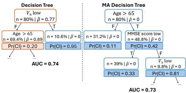
Take a look at Figure 1 above. On the left is a standard Decision Tree. It achieves an AUC (accuracy metric) of 0.74. However, its very first question relies on “Hippocampal Volume” (\(V_h\)), a value derived from an MRI scan. In this dataset, that value is missing for 77% of patients (\(\hat{\rho} = 0.77\)). If the patient hasn’t had an MRI, the model relies on imputed values or a default path, which is risky.

On the right is a Missingness-Avoiding (MA) Tree. It achieves nearly the same accuracy (AUC 0.73) but starts by asking for “Age”—a value that is almost never missing. It only asks for the MRI scan if the patient is over 65 and has a low cognitive score. For many patients, it never needs to ask for the MRI at all. This model has “learned” that the MRI is frequently missing and structured its decision logic to avoid it whenever possible.

The MA Framework: A New Objective

How do we mathematically force a model to behave like the tree on the right? The authors introduce a new regularization term to the standard loss function.

Usually, we train models to minimize the difference between the prediction and the true label (the Loss, \(L\)). The authors add a penalty for Missingness Reliance (\(\rho\)).

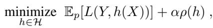
Here, \(\alpha\) (alpha) is a hyperparameter that controls the trade-off.

• If \(\alpha = 0\), the model ignores missingness and focuses only on accuracy (standard behavior).
• As \(\alpha\) increases, the model is penalized more heavily for relying on features that are likely to be missing at test time.

Defining Missingness Reliance (\(\rho\))

But what exactly is \(\rho\)? It is defined as the probability that the model needs a value that turns out to be “na” (not available).

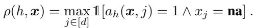
In simple terms, for a specific input \(\mathbf{x}\), if the model’s logic path requires feature \(j\) (\(a_h(\mathbf{x}, j) = 1\)), and feature \(j\) happens to be missing (\(x_j = \mathbf{na}\)), then the reliance is 1. Otherwise, it is 0.

The goal is to minimize the expected value of this reliance across the entire dataset.

Strategies for Avoidance

The paper identifies three main ways a model can avoid missing values, visualized below:

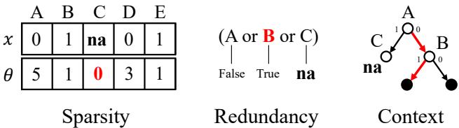
1. Sparsity (Left): The model simply stops using features that are frequently missing. This is common in linear models like LASSO.
2. Redundancy (Middle): The model learns alternative rules. If \(A\) is missing, check if \(B\) or \(C\) can provide the same information.
3. Context (Right): This is where decision trees shine. The model changes the order of questions. It only asks for a potentially missing feature (like an MRI result) in specific contexts (branches) where it is absolutely necessary and likely to be available.

Let’s dive into how the researchers implemented this for specific algorithms.

1. MA-DT: Missingness-Avoiding Decision Trees

Decision trees are naturally suited for contextual avoidance. A standard decision tree splits data based on criteria like Gini impurity. The MA-DT modifies this splitting criterion.

When evaluating a potential split on feature \(j\), the algorithm calculates the standard impurity reduction but subtracts a penalty proportional to how often feature \(j\) is missing in the current node.

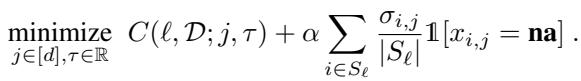
In this equation:

• \(C\) is the standard cost (impurity).
• \(\alpha\) is our regularization strength.
• The summation counts how many samples in the current node (\(S_{\ell}\)) have a missing value for feature \(j\).

This simple change forces the tree to prefer splits on “safe,” available features (like Age or Sex) higher up in the tree, pushing the “risky,” frequently missing features deeper down, where they apply to fewer samples.

2. MA-LASSO: Sparse Linear Models

For linear models (like Logistic Regression), “context” doesn’t exist. You essentially use all selected features at once. Here, avoidance relies on sparsity.

The authors modify the classic LASSO (L1 regularization) objective. Standard LASSO penalizes the absolute size of coefficients (\(|\theta|\)) to drive irrelevant features to zero. MA-LASSO weights this penalty by the missingness rate of each feature.

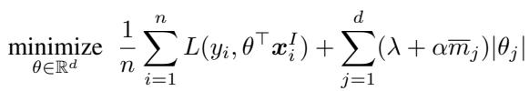
Here, \(\bar{m}_j\) is the fraction of times feature \(j\) is missing. If a feature is missing 90% of the time, its penalty is massive. The model will try very hard to set its coefficient \(\theta_j\) to zero, effectively removing it from the equation unless it is incredibly predictive.

Theoretical Insight: ODDC Rules

One of the most fascinating contributions of the paper is the formalization of Observed Deterministic Data Collection (ODDC) rules.

In many systems, data isn’t missing at random; it’s missing by design.

• Example: A “Pregnancy Test Result” variable is always missing for male patients.
• Example: A “Follow-up Lab Result” is only present if the “Initial Screen” was positive.

The authors define an ODDC rule as an implication: “If variables \(X_T\) have values in set \(A\), then variable \(j\) is observed.”

Why does this matter? The authors prove that if the outcome \(Y\) depends on the input \(X\) through these rules, it is theoretically possible to build a model with zero missingness reliance (\(\rho=0\)) without sacrificing predictive accuracy.

An MA-DT (Decision Tree) is perfect for this. By adjusting \(\alpha\), the tree naturally learns the structure of the data collection process. It learns to check “Sex” before asking for “Pregnancy Test,” or check “Initial Screen” before asking for “Lab Result.”

Experiments and Results

The researchers tested their framework on six real-world healthcare and finance datasets, including NHANES (hypertension prediction) and ADNI (Alzheimer’s diagnosis). They compared MA models against standard baselines (Logistic Regression, Random Forest, XGBoost) using different imputation strategies.

Key Finding: The “Free Lunch”

The results show that you can often drastically reduce reliance on missing values with little to no drop in accuracy (AUROC).

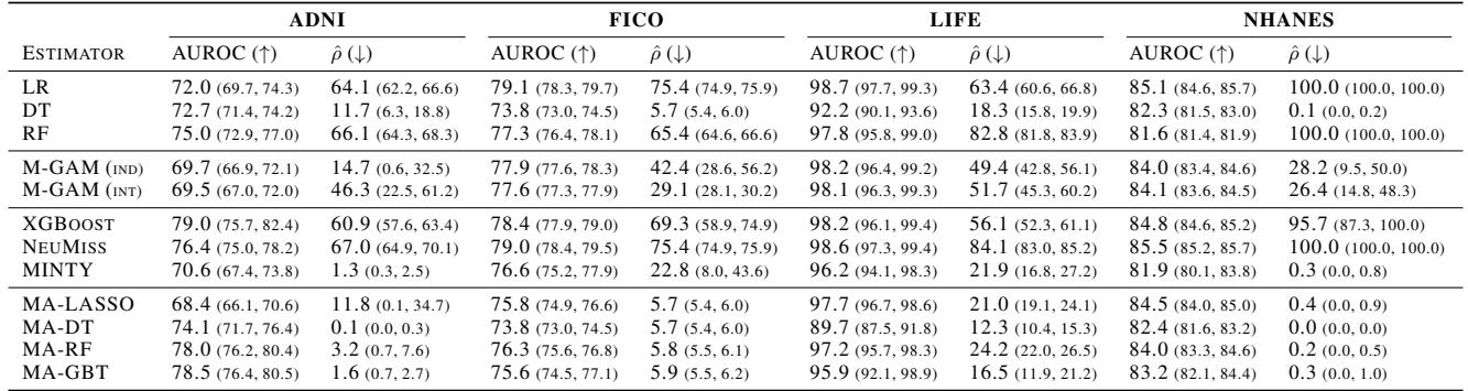
Looking at Table 1:

• In the NHANES dataset, a standard Logistic Regression (LR) relies on missing values 100% of the time (\(\hat{\rho} = 100.0\)).
• The MA-LASSO model achieves comparable accuracy (AUROC ~84.5 vs 85.1) but reduces missingness reliance to just 0.4%.
• Similarly, for ADNI, the standard Decision Tree (DT) has a reliance of 11.7%, while MA-DT reduces this to 0.1% with a slightly higher AUC (74.1 vs 72.7).

This confirms the hypothesis: standard models are “lazy.” They grab messy features because they provide a marginal gain during training, ignoring the cost of missingness. MA models force them to find cleaner, more robust paths.

The Trade-off Curve

Of course, sometimes avoiding missing data does cost accuracy. The parameter \(\alpha\) allows practitioners to navigate this trade-off.

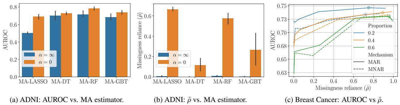
In Figure 4 (c) (the curve on the right), we see the performance of MA-LASSO on the Breast Cancer dataset with synthetic missingness.

• As we allow more missingness reliance (moving right on the x-axis), the accuracy (AUROC) improves.
• However, the curve is steep at the beginning and then flattens. This means we can eliminate a huge amount of missingness reliance for a very small “price” in accuracy.

Interpreting the Models

A major advantage of MA models, particularly trees, is interpretability. We can visualize exactly how the model navigates around missing data.

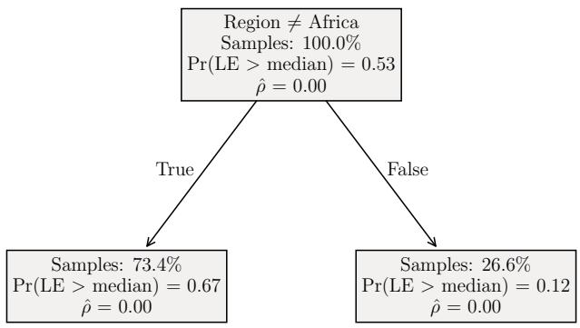
Figure 6 shows three trees trained on the LIFE dataset (predicting life expectancy):

1. (a) \(\alpha = 0\) (Standard Tree): Splits immediately on “Adult Mortality” and “Infant Deaths.” If these are missing, the model is stuck.
2. (b) \(\alpha = \alpha^*\) (Balanced MA-Tree): Splits on “Adult Mortality” first, but then uses “Region” (which is never missing) to handle cases where mortality data might be spotty. It balances accuracy with availability.
3. (c) \(\alpha = \infty\) (Maximum Avoidance): Splits only on “Region.” It never asks for mortality data. This has zero missingness reliance (\(\rho=0\)) but, as expected, lower accuracy (AUC 0.67 vs 0.90).

The middle ground (b) is usually where the magic happens.

Conclusion

The “Missingness-Avoiding” framework offers a compelling shift in how we think about supervised learning with incomplete data. Rather than viewing missing values as a data cleaning problem to be solved before modeling (via imputation), the authors treat it as a modeling constraint to be solved during training.

For students and practitioners, the takeaways are clear:

1. Imputation isn’t innocent: It introduces bias and opacity.
2. Context matters: In trees, the order of features determines whether you need a missing value or not.
3. You have a choice: You don’t have to accept a model that relies on data you might not have. By penalizing missingness reliance, you can build models that are robust, interpretable, and “test-time safe.”

This approach gives us models that don’t just predict the future—they understand the limitations of the present data, making them far safer for deployment in the real world.