Introduction

In the world of time series forecasting—whether we are predicting stock prices, hospital admission rates, or electricity demand—knowing what will happen is only half the battle. The other, often more critical half, is knowing how sure we are about that prediction.

Imagine an AI predicting traffic flow. A prediction of “50 cars per minute” is useful. But a prediction of “50 cars per minute, give or take 5 cars” leads to very different decision-making than “50 cars per minute, give or take 40 cars.” This is the domain of probabilistic time series forecasting.

Recently, Denoising Diffusion Probabilistic Models (DDPMs)—the same tech behind image generators like DALL-E and Stable Diffusion—have shown incredible promise in this field. They are excellent at generating complex distributions. However, they suffer from a significant flaw when applied to real-world data: they generally assume that the “noise” (uncertainty) in the data is constant or follows a simple, fixed pattern.

In reality, data is non-stationary. The volatility of a stock market changes during a crash; the variance in flu cases explodes during an outbreak. Standard diffusion models struggle to adapt to these changing levels of uncertainty.

In this post, we will dive deep into a new research paper, “Non-stationary Diffusion For Probabilistic Time Series Forecasting” (NsDiff). We will explore how this novel framework ditches the rigid assumptions of traditional models, enabling it to dynamically adapt to the changing chaos of the real world.

The Problem: When Physics Meets Statistics

To understand why NsDiff is necessary, we first need to look at how diffusion models typically handle time series.

General forecasting methods train a model \(f(\mathbf{X})\) to predict a future series \(\mathbf{Y}\). This usually gives us the conditional expectation, or the “average” outcome. To get the probability distribution (the uncertainty), diffusion models add noise to the data and then learn to reverse that process.

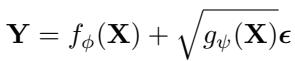
Most existing DDPMs rely on the Additive Noise Model (ANM). They assume:

Here, \(\boldsymbol{\epsilon}\) represents stationary Gaussian noise \(\mathcal{N}(\mathbf{0}, \mathbf{I})\). In plain English, this model assumes that while the trend (the mean) might change based on the input \(\mathbf{X}\), the uncertainty (the variance of the noise) is fixed and unchanging.

Visualizing the Failure Mode

This assumption breaks down in high-stakes scenarios. Consider predicting the number of patients with an influenza-like illness (ILI). As the season peaks, not only does the number of patients rise, but the unpredictability of that number also rises.

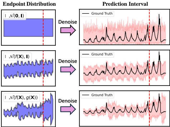
Figure 1 above perfectly illustrates this limitation:

• Top Row (TimeGrad): This model assumes a standard Gaussian endpoint \(\mathcal{N}(0, \mathbf{I})\). Notice how the prediction interval (the pink shaded area) on the right is uniform and fails to capture the rising trend or the expanding uncertainty.
• Middle Row (TMDM): This model improves things by targeting a changing mean \(\mathcal{N}(f(\mathbf{X}), \mathbf{I})\). It captures the trend (the curve goes up), but the width of the pink interval stays constant. It essentially thinks the prediction is just as “safe” at the peak of the outbreak as it was at the start.
• Bottom Row (NsDiff - Our Focus): This model targets \(\mathcal{N}(f(\mathbf{X}), g(\mathbf{X}))\). It captures both the rising trend and the expanding uncertainty. The pink interval widens as the situation becomes more volatile.

The Core Method: Non-stationary Diffusion (NsDiff)

The researchers propose a solution called NsDiff. The core innovation lies in relaxing the rigid Additive Noise Model and replacing it with a Location-Scale Noise Model (LSNM).

1. The Location-Scale Noise Model (LSNM)

Instead of adding fixed noise, NsDiff models the future series using a more flexible equation:

In this equation:

• \(f_{\phi}(\mathbf{X})\) models the conditional expectation (the trend).
• \(g_{\psi}(\mathbf{X})\) models the varying uncertainty (the variance).
• \(\epsilon\) is standard Gaussian noise.

By introducing \(g_{\psi}(\mathbf{X})\), the model acknowledges that the “scale” of the noise depends on the input data \(\mathbf{X}\). If the input suggests a volatile period (like a holiday rush in traffic data), \(g_{\psi}(\mathbf{X})\) will be large. If the input suggests a calm period, it will be small.

Both \(f_{\phi}\) and \(g_{\psi}\) are implemented as pre-trained neural networks (like Transformers or MLPs) that provide “prior knowledge” to the diffusion process.

2. The NsDiff Framework

How do we actually train a diffusion model to respect this new noise model? The authors designed a framework that integrates an uncertainty-aware noise schedule.

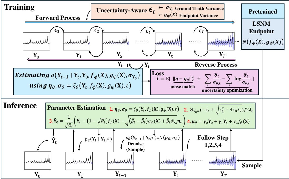
As shown in Figure 2, the process involves two main phases:

1. Training (Top): We take the ground truth \(\mathbf{Y}_0\) and gradually add noise until it reaches a target distribution \(\mathbf{Y}_T\). Crucially, unlike standard DDPMs where \(\mathbf{Y}_T\) is random noise, here \(\mathbf{Y}_T\) is derived from our priors \(f_{\phi}(\mathbf{X})\) and \(g_{\psi}(\mathbf{X})\).
2. Inference (Bottom): We start by sampling from our predicted endpoint distribution (using the priors) and iteratively denoise it to generate the final prediction.

3. The Uncertainty-Aware Noise Schedule

This is where the mathematics gets clever. In a standard diffusion model, you add noise according to a fixed schedule \(\beta_t\). In NsDiff, the noise added at each step must account for the fact that we are moving toward a specific, data-dependent variance \(g_{\psi}(\mathbf{X})\).

The forward process distribution \(q(\mathbf{Y}_t | \mathbf{Y}_{t-1})\) is modified. The distribution of the noisy data at any step \(t\) is calculated as:

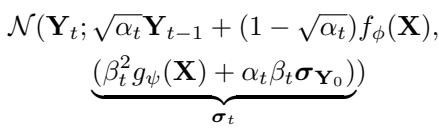
Look closely at the variance term \(\pmb{\sigma}_t\) in the equation above. It is a weighted combination of the predicted variance \(g_{\psi}(\mathbf{X})\) and the actual data variance \(\sigma_{\mathbf{Y}_0}\).

• As \(t \to T\) (more noise), the variance converges to our estimated \(g_{\psi}(\mathbf{X})\).
• As \(t \to 0\) (less noise), it reflects the actual data.

This dynamic adjustment allows the diffusion process to “bridge” the gap between the clean data and the complex, non-stationary endpoint we want to model.

4. The Reverse Process & Loss Function

The goal of the reverse process (denoising) is to estimate the noise \(\boldsymbol{\eta}\) that was added. The neural network \(\xi_{\theta}\) takes the noisy step \(\mathbf{Y}_t\), the priors \(f_{\phi}\) and \(g_{\psi}\), and the time step \(t\) as input.

The loss function used to train this network is interesting because it doesn’t just look at the error in the noise; it also optimizes for the variance:

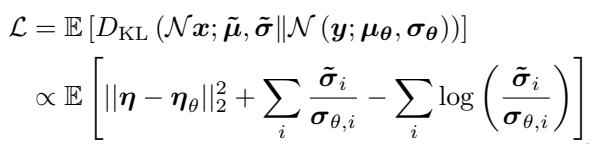
The first term \(||\boldsymbol{\eta} - \boldsymbol{\eta}_{\theta}||^2\) ensures the mean is estimated correctly (standard in DDPMs). The summation terms on the right specifically penalize errors in variance estimation, forcing the model to pay attention to the scale of the uncertainty.

5. Inference: The Quadratic Solution

Here is a fascinating technical detail. To perform the reverse denoising steps accurately, the model needs to know the variance of the original data, \(\sigma_{\mathbf{Y}_0}\).

During training, we know the ground truth \(\mathbf{Y}_0\), so calculating its variance is trivial. But during inference (predicting the future), we don’t have \(\mathbf{Y}_0\).

We could just use our predictor \(g_{\psi}(\mathbf{X})\), but that blindly trusts the pre-trained model and ignores what the diffusion model sees during the reverse process. Instead, the authors derive a relationship between the estimated noise variance \(\sigma_{\theta}\) and the ground truth variance.

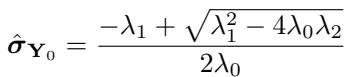
It turns out this relationship forms a quadratic equation:

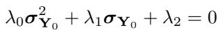
By solving this quadratic equation for \(\sigma_{\mathbf{Y}_0}\), the model can dynamically estimate the variance of the target data during the generation process.

This allows NsDiff to refine its understanding of the uncertainty as it generates the sample, rather than relying solely on the initial guess from the pre-trained model.

Experiments & Results

The authors tested NsDiff on nine real-world datasets (including Electricity, Traffic, and Exchange Rate) and synthetic datasets designed to stress-test uncertainty handling.

Real-World Performance

They compared NsDiff against strong baselines like TimeGrad, CSDI, and TMDM. The metrics used were CRPS (Continuous Ranked Probability Score - measuring accuracy of the distribution) and QICE (Quantile Interval Coverage Error - measuring how well the predicted intervals cover the true data). Lower is better for both.

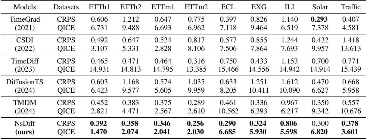
As shown in Table 3, NsDiff achieves state-of-the-art results across almost all datasets.

• On the Traffic dataset, which has extremely high uncertainty variation, NsDiff reduces the QICE score by 66.3% compared to TMDM.
• On ETTh1 and ETTh2 (electricity transformer data), it reduces QICE by roughly 50%.

Visual Confirmation

Numbers are great, but time series forecasting needs to be seen to be believed. Let’s look at a sample from the ETTh1 dataset.

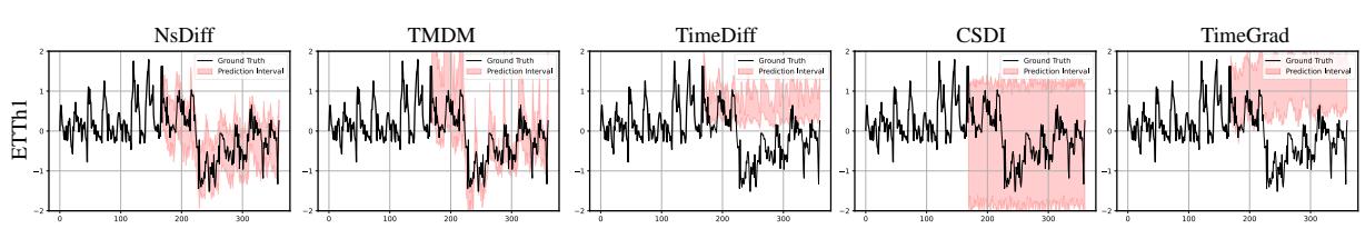
In Figure 3:

• TimeGrad and CSDI (Right) struggle significantly. TimeGrad predicts a flat trend when the reality is a sharp drop.
• TMDM (Second from Left) captures the drop in the mean (black line), but look at the pink interval. It’s a constant width tube. It doesn’t acknowledge that the drop might introduce more volatility.
• NsDiff (Left) captures the drop and provides a tight, accurate prediction interval that hugs the ground truth.

The Synthetic Stress Test

To rigorously prove that NsDiff handles changing variance better, the researchers created synthetic datasets where the variance grows linearly or quadratically over time.

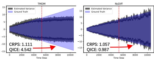
Figure 4 is the “smoking gun.”

• The Left chart (TMDM) shows the model effectively “giving up” on the variance shift. After the red dashed line (the test set), the predicted variance (grey line) goes flat, completely missing the fact that the ground truth variance (blue shading) is increasing.
• The Right chart (NsDiff) tracks the increasing variance almost perfectly. It understands that the environment has changed and adapts its uncertainty estimates accordingly.

Conclusion and Implications

The NsDiff paper highlights a crucial gap in generative time series forecasting: the assumption of stationarity in uncertainty. By sticking to the Additive Noise Model, previous state-of-the-art models were essentially wearing blinders, capable of seeing where the trend was going but blind to how risky the prediction was becoming.

By integrating the Location-Scale Noise Model (LSNM) and deriving a mathematically rigorous uncertainty-aware noise schedule, NsDiff offers a generalized framework. It essentially says: “Let’s use the power of diffusion models, but let’s guide them with explicit, adaptive priors about the mean and variance.”

For students and practitioners, this paper serves as an excellent lesson in inductive bias. A powerful generic model (like a standard DDPM) often loses out to a model that incorporates specific knowledge about the problem structure (like the fact that variance changes over time). As we move toward using AI for critical infrastructure and financial decision-making, tools like NsDiff that can honestly and accurately report their own uncertainty will be indispensable.