Introduction

In the world of machine learning, Time-Series Classification (TSC) is a ubiquitous challenge. From detecting heart arrhythmias in ECG signals to recognizing gestures from smartwatches or classifying robot movements on different surfaces, time-series data is everywhere.

However, practitioners often face a difficult trade-off: Accuracy vs. Interpretability.

Deep neural networks generally provide the highest accuracy, acting as powerful “black boxes” that ingest data and output predictions. But in critical fields like healthcare, a “black box” isn’t enough. A doctor needs to know why a model thinks a heartbeat is irregular. This is where Shapelets come in. Shapelets are specific, discriminative subsequences—little “shapes” within the data—that act as signatures for a class. While highly interpretable, discovering them is computationally expensive, and traditional methods often discard a vast amount of potentially useful contextual information to save time.

What if we didn’t have to choose between the efficiency of discarding data and the accuracy of keeping it?

In this post, we explore a new research paper, “Learning Soft Sparse Shapes for Efficient Time-Series Classification,” which introduces SoftShape. This model proposes a novel “soft” sparsification mechanism. Instead of ruthlessly deleting less informative shapes, it intelligently weights and fuses them, preserving vital context while maintaining efficiency.

Let’s look at a concrete example provided by the researchers.

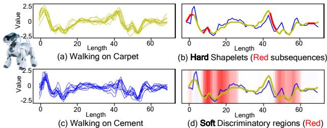
In the image above, (a) and (c) show raw sensor data from a robot dog walking on carpet versus cement. Traditional “hard” shapelet methods (b) identify specific red subsequences as important and ignore the rest. However, this misses the subtle patterns in the non-red areas. The proposed SoftShape method (d) highlights discriminative regions with a “soft” red shading, capturing a much richer, more nuanced view of what makes the “Carpet” class unique.

The Problem: Hard Decisions in a Nuanced World

To understand SoftShape, we first need to understand the limitation it solves.

A time series \(\mathcal{X}\) is a sequence of data points ordered by time. A subsequence is a smaller slice of that series. If a specific subsequence (like a sudden spike or a sine wave pattern) appears frequently in Class A but not Class B, it is a Shapelet.

Traditionally, identifying shapelets involves a brute-force search or a “hard” selection process:

1. Extract all possible subsequences.
2. Score them based on how well they split the classes.
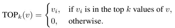
3. Keep the top \(k\) (the most discriminative ones).
4. Discard the rest.

This is called Hard Sparsification. Ideally, this leaves you with a small, efficient set of features. Practically, it creates two problems:

1. Information Loss: The “rejected” subsequences might contain weak but useful signals, especially for complex classifications where context matters.
2. Binary Importance: A subsequence is treated as either “critical” or “useless,” ignoring the reality that some parts of a signal are “somewhat” important.

SoftShape aims to replace this hard filtering with Soft Sparsification.

The SoftShape Architecture

The SoftShape model is designed to act like a human expert reading a chart: it focuses intently on the important spikes (discriminative shapes) but still keeps an eye on the background noise (fused non-discriminative shapes) for context.

Here is the high-level architecture:

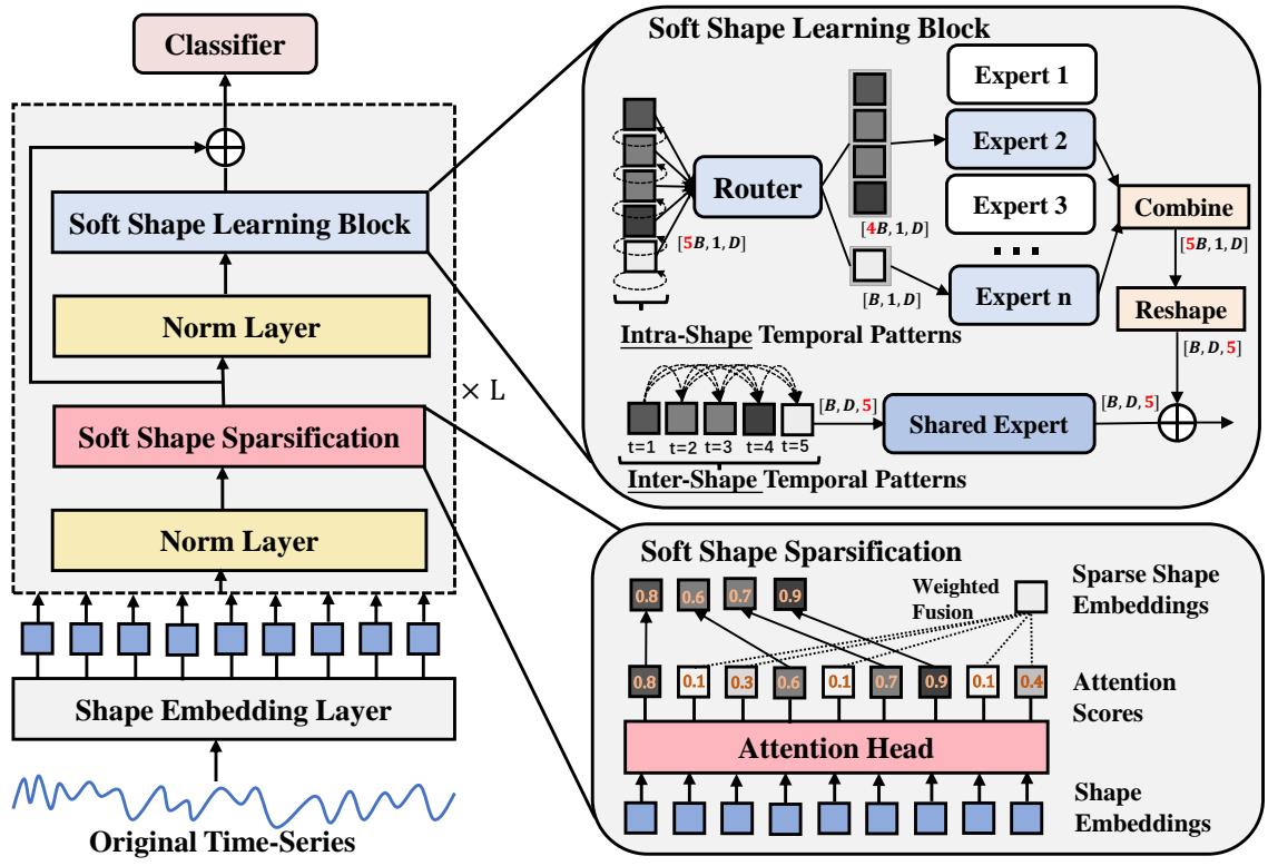
The model consists of three main stages:

1. Shape Embedding: Converting raw time points into feature vectors.
2. Soft Shape Sparsification: The core innovation—weighting and fusing shapes.
3. Soft Shape Learning Block: Using advanced neural components to learn patterns within and between shapes.

Let’s break these down step-by-step.

1. Shape Embedding and Attention

First, the model needs to process the raw time series. Instead of looking at single time points, it looks at overlapping windows (subsequences).

The set of all possible subsequences \(\mathcal{A}\) is mathematically defined as:

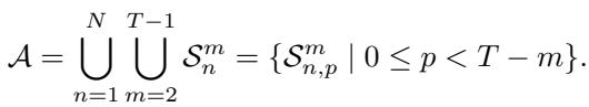
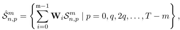
The model uses a 1D Convolutional Neural Network (CNN) to transform these raw subsequences into Shape Embeddings. Each window of the time series is converted into a dense vector \(\hat{S}\).

Scoring the Shapes

Once we have these shape embeddings, how do we know which ones are important? The model employs a learnable Attention Head. This is a small neural network layer that looks at a shape embedding and outputs a score \(\alpha\) between 0 and 1. A score close to 1 means the shape is highly discriminative; a score close to 0 means it’s likely noise or irrelevant background.

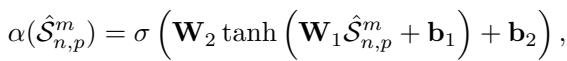
2. Soft Shape Sparsification: The “Weighted Fusion”

This is where SoftShape diverges from traditional methods. Instead of setting a threshold and deleting everything below it, SoftShape performs a Soft Split.

The model ranks all shapes based on their attention scores. It then defines a proportion \(\eta\) (e.g., top 50%).

For the Top \(\eta\) Shapes (The “Stars”): These shapes are kept distinct. However, they are scaled by their attention score. This emphasizes the most confident predictions.

For the Bottom \((1-\eta)\) Shapes (The “Background”): In a hard approach, these would be deleted. in SoftShape, they are fused. The model calculates a weighted sum of all these low-score shapes to create a single Fused Shape.

This results in a new sequence of shapes: the original high-scoring ones (scaled), plus one single shape that represents the aggregate information of everything else. This reduces the computational load significantly (we are processing fewer shapes) without completely blinding the model to the background context.

3. Soft Shape Learning Block

Now that we have a sparse but informative set of shapes, the model needs to learn from them. The researchers introduce a dual-pathway learning block that captures two types of patterns: Intra-Shape (patterns inside a single shape) and Inter-Shape (relationships between different shapes over time).

Intra-Shape Learning: Mixture of Experts (MoE)

Different shapes represent different physical events (e.g., a “step” vs. a “stumble”). A single neural network might struggle to be good at analyzing all of them.

SoftShape uses a Mixture of Experts (MoE). This is a collection of small, specialized networks (“experts”). A Router looks at each shape and decides which expert is best suited to handle it.

To ensure efficiency, the router only activates the Top-\(k\) experts (usually just 1 or 2) for any given shape.

The output is processed by the selected expert. This allows the model to specialize—Expert A might become really good at recognizing “upward slopes,” while Expert B specializes in “flat plateaus.”

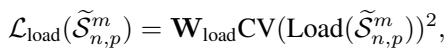
To prevent the router from getting lazy and always choosing the same expert (which would leave others untrained), the researchers include load-balancing loss functions during training:

Inter-Shape Learning: The Shared Expert

While the MoE looks at shapes in isolation, time-series data is sequential. The order matters. To capture this, the model reassembles the sparsified shapes into a sequence.

A Shared Expert (implemented as an Inception-based CNN) scans across this sequence. It learns discriminative features based on the evolution of shapes over time—capturing the global temporal patterns that individual shapelets miss.

4. Classification

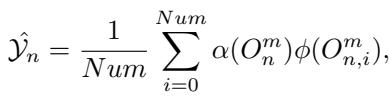
Finally, the outputs from the intra-shape and inter-shape paths are combined. The model calculates the final class probability by aggregating the weighted votes of the processed shapes.

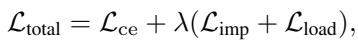
The model is trained end-to-end using a total loss function that combines standard Cross-Entropy loss (for accuracy) with the auxiliary losses (for expert load balancing).

Experimental Results

Does this “soft” approach actually work better than “hard” selection or standard deep learning? The researchers tested SoftShape on the massive UCR Time Series Archive (128 datasets).

Accuracy Comparison

The results were compelling. SoftShape demonstrated superior performance compared to a wide range of baselines, including CNNs, Transformers, and Foundation Models.

The critical difference diagram below visualizes the statistical ranking of the methods. Methods connected by a horizontal bar are not statistically different, while those further to the right are statistically superior.

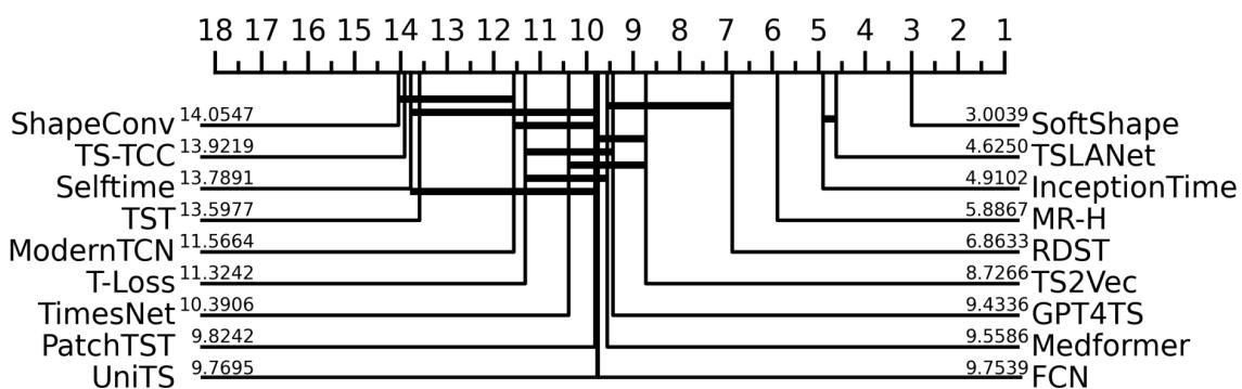
SoftShape (at the far right) achieves the best average rank (lowest number is best), significantly outperforming popular models like InceptionTime, PatchTST, and RDST.

Efficiency

One of the main promises of “sparsification” is efficiency. By fusing the non-essential shapes, the model has less data to process in the deep layers.

The chart below compares the running time (training speed) of SoftShape against other deep learning models on two datasets (ChlorineConcentration and HouseTwenty).

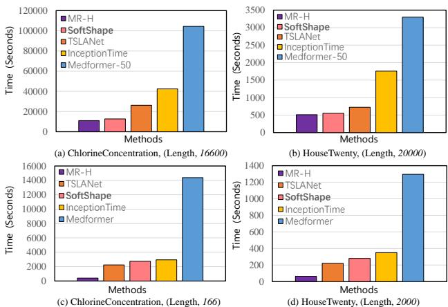
SoftShape (orange bars) is consistently faster than heavy Transformer models like Medformer and competitive with efficient CNNs like TSLANet, especially as the sequence length increases (Figures 3a and 3b).

Interpretability

Can we understand what the model is learning? Using Multiple Instance Learning (MIL) visualization, the researchers plotted which parts of a time series SoftShape focused on.

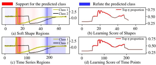
In Figure 4(d), the red line represents the “learning score” (attention). We can see the model places high attention on the specific peaks and troughs that characterize the class, while the flat “noise” areas receive lower scores. This confirms that SoftShape is successfully identifying discriminative regions.

Clustering Power (t-SNE)

To see how well the model separates classes, the researchers visualized the shape embeddings.

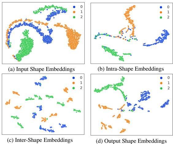
• (a) Input: The raw shape embeddings are messy and overlapping.
• (b) Intra-Shape: The MoE starts to group similar structures.
• (c) Inter-Shape: The global learner separates distinct temporal patterns.
• (d) Output: The final embeddings show distinct, well-separated clusters corresponding to the three classes (Blue, Orange, Green). This clean separation makes the final classification task much easier for the linear classifier.

Does every part matter? (Ablation Study)

The researchers stripped the model down to see which components contributed the most.

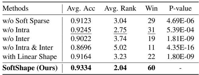
• w/o Soft Sparse: Removing soft sparsification (using hard selection instead) dropped accuracy significantly.
• w/o Intra / w/o Inter: Removing either the MoE or the Shared Expert caused performance drops, proving that both local shape specialization and global sequence modeling are necessary.

Conclusion

The SoftShape model represents a smart evolution in time-series classification. It addresses the “black box” problem of deep learning without sacrificing the performance that modern applications demand.

By introducing Soft Sparsification, the authors showed that we don’t need to throw away data to be efficient; we just need to compress the “boring” parts intelligently. Furthermore, by combining Intra-shape MoE (specialized local analysis) with Inter-shape learning (global sequence analysis), SoftShape captures the full complexity of time-series data.

For students and practitioners, this paper highlights a crucial lesson: how we represent data (embeddings and sparsification) is often just as important as the model architecture itself.

The code for SoftShape is open-source and available, offering a new tool for anyone looking to build interpretable, efficient, and accurate time-series models.