Introduction

Imagine you are handed a spreadsheet with two columns of data: Column A and Column B. You plot them, and they are perfectly correlated. As Column A increases, Column B increases.

Now, answer this question: Does A cause B, or does B cause A?

This is one of the most fundamental challenges in science, economics, and artificial intelligence. We have all heard the mantra “correlation does not imply causation.” Usually, to figure out the direction of causality, we rely on interventions—we poke the system (like a randomized controlled trial in medicine) and see what breaks.

But what if you can’t poke the system? What if you only have observational data, like historical stock prices or telescope readings from a distant galaxy?

In the paper “Identifying Causal Direction via Variational Bayesian Compression,” researchers Quang-Duy Tran and colleagues propose a fascinating solution that bridges deep learning, information theory, and statistics. They argue that the “true” causal direction is simply the one that allows for the most efficient compression of the data.

To achieve this, they introduce a method called COMIC (COmpression-based method for Identifying Causal direction). By using Bayesian Neural Networks to model the relationship between variables, they calculate which causal direction describes the data most succinctly.

In this post, we will tear down this paper to understand why “simplicity” implies causality, how we can measure the complexity of a neural network, and why this new method outperforms traditional statistical approaches.

Background: The Philosophy of Compression

To understand how a computer can determine if rain causes wet grass (and not the other way around) just by looking at numbers, we need to visit the concept of Kolmogorov Complexity.

The Algorithmic Markov Condition

The foundational idea here is Occam’s Razor: the simplest explanation is usually the correct one. In information theory, this is formalized as the Kolmogorov Complexity, which is the length of the shortest computer program required to generate a specific dataset.

The researchers base their work on the Algorithmic Markov Condition. This postulate states that if \(X\) causes \(Y\) (denoted \(X \to Y\)), then the mechanism generating \(X\) and the mechanism generating \(Y\) from \(X\) are independent “modules” of nature.

If we try to describe the joint distribution of both variables, \(P(X, Y)\), the true causal direction yields the most efficient factorization.

In the equation above, \(K(\cdot)\) represents the complexity (or description length). The equation says that the complexity of the pair \((X, Y)\) is roughly equal to the complexity of the cause \(X\) plus the complexity of the effect \(Y\) given the cause.

Here is the kicker: This relationship is asymmetric.

If \(X \to Y\) is the true direction, factorization in that direction is “clean.” However, if we try to factorize it in the anti-causal direction (\(Y \to X\)), the terms \(P(Y)\) and \(P(X|Y)\) become simpler to describe together than apart because they share information. The universe doesn’t generate the effect first; if you force a model to think it does, the mathematical description becomes messy and bloated.

Therefore, we can test for causality by checking which direction produces a shorter description:

If the left side of the inequality is smaller, \(X\) causes \(Y\). If the right side is smaller, \(Y\) causes \(X\).

The Problem with “Ideally” Simple

There is a catch. Kolmogorov Complexity is theoretically computable but practically impossible. You cannot calculate the “absolute shortest program” for any arbitrary data because of the Halting Problem.

So, researchers rely on the Minimum Description Length (MDL) principle. Instead of finding the perfect program, we try to find the best model from a specific class of models. We calculate the “codelength” (or file size) required to transmit the data.

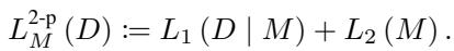
In MDL, the total codelength consists of two parts:

1. Model Cost (\(L_2\)): How many bits does it take to describe the model’s parameters?
2. Data Cost (\(L_1\)): How well does the model fit? (If the model fits perfectly, the “error” residuals are small and cheap to encode. If the model fits poorly, the errors are large and expensive to encode.)

This creates a tradeoff. You can fit the data perfectly with a super-complex model (high Model Cost, low Data Cost), or you can use a simple model that fits poorly (low Model Cost, high Data Cost). The “true” causal direction is the one that minimizes the sum of these two.

Why Previous Methods Failed

Before this paper, researchers used simple regression models (like linear regression) to estimate these codelengths. But the real world isn’t linear. If the relationship between \(X\) and \(Y\) is a complex sine wave or a jagged polynomial, simple models fail to capture the fit, leading to inaccurate codelengths.

Others tried Gaussian Processes (GPs), which are flexible but computationally incredibly expensive (\(O(N^3)\)), making them useless for large datasets.

This brings us to the authors’ proposal: Neural Networks.

Core Method: COMIC

The method introduced in this paper is COMIC. It stands for a Bayesian COMpression-based approach to Identifying the Causal direction.

The authors propose using Neural Networks because they are “universal approximators”—they can model any relationship, linear or non-linear. However, standard Neural Networks are prone to overfitting. If you use a massive network, it will memorize the data. Its “Data Cost” (error) will be zero, but its “Model Cost” (complexity) should theoretically be huge.

The problem is, in standard Deep Learning, we don’t usually measure the “file size” of the weights. We just minimize error.

To solve this, the authors utilize Variational Bayesian (VB) Learning.

Variational Bayesian Code

How do you calculate the file size of a Neural Network? You treat the weights not as fixed numbers, but as probability distributions.

In a Bayesian Neural Network, every weight \(w\) is a bell curve (Gaussian distribution) defined by a mean \(\mu\) and a variance \(\sigma^2\).

• If the variance is tight, the weight is precise (requires more information/bits to encode).
• If the variance is wide, the weight is vague (requires fewer bits).

The authors use a coding scheme called Bits-Back Coding (conceptually similar to the Variational Evidence Lower Bound or ELBO). The total codelength for the conditional distribution \(Y|X\) is approximated by minimizing the following objective:

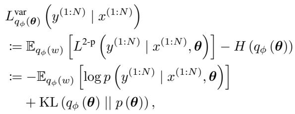
Let’s break down this crucial equation:

1. The First Term (Data Fitness): \(-\mathbb{E}[\log p(y|x, \theta)]\). This measures how well the network predicts \(Y\) given \(X\). It essentially looks at the likelihood of the data. If the prediction is good, this number is low.
2. The Second Term (Model Complexity): \(KL(q_\phi(\theta) || p(\theta))\). This is the Kullback-Leibler Divergence. It measures the “distance” between the learned posterior distribution of the weights \(q_\phi\) and a simple prior distribution \(p(\theta)\) (usually a standard Gaussian).

Think of the Prior \(p(\theta)\) as the “default” state of the model (random noise). The KL term measures how much “information” the model had to learn to move away from that random state to fit the data. This effectively calculates the model complexity (\(L_2\)) in bits (or nats).

The Architecture of the Cause

COMIC determines the direction by comparing two models:

1. Forward Model: Assume \(X\) causes \(Y\).

• Encode \(X\) using a standard marginal distribution (cost = \(L_{marginal}(X)\)).
• Train a Bayesian Neural Network to predict \(Y\) from \(X\).
• Calculate the VB codelength (cost = \(L_{conditional}(Y|X)\)).

2. Backward Model: Assume \(Y\) causes \(X\).

• Encode \(Y\) using a standard marginal distribution.
• Train a Bayesian Neural Network to predict \(X\) from \(Y\).
• Calculate the VB codelength.

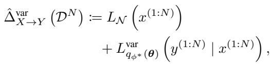
The total score for the direction \(X \to Y\) is the sum of the marginal and conditional parts:

The neural network itself isn’t just a standard regressor. It models Heteroscedasticity (varying noise). In causal discovery, the “noise” or “error” often changes depending on the input value. To capture this, the network outputs two values for every input: the predicted mean (\(\mu\)) and the predicted noise variance (\(\sigma\)).

Here, \(f_{Y,1}\) predicts the value of \(Y\), and \(f_{Y,2}\) predicts the uncertainty (standard deviation) of that prediction. \(\zeta\) is a function that ensures the variance is always positive (like a Softplus function).

The Causal Indicator Score

Once the models are trained in both directions, we simply compare the scores. The authors define the causal indicator \(\hat{\Delta}^{\text{var}}\):

• If \(\hat{\Delta}^{\text{var}}\) is positive, it means the \(X \to Y\) codelength is smaller (better). We conclude \(X\) causes \(Y\).
• If \(\hat{\Delta}^{\text{var}}\) is negative, it means the \(Y \to X\) codelength is smaller. We conclude \(Y\) causes \(X\).
• The magnitude of the number tells us the confidence. A result near zero means the method is “indecisive.”

Why This is Indentifiable

One of the major theoretical contributions of this paper is proving identifiability.

In many statistical models (like linear Gaussian models), the math works out identically in both directions—you can’t tell the difference. This is called “distribution equivalence.”

The authors prove that their specific setup (Bayesian Neural Networks with Gaussian priors) is non-separable-compatible.

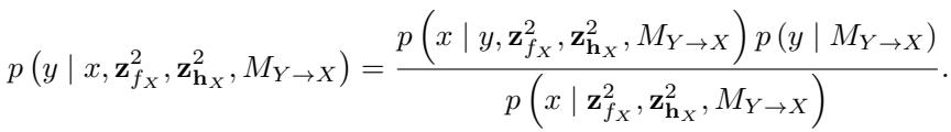
Without getting bogged down in the density of the proof, the gist is this: If you generate data with a neural network in the forward direction (\(X \to Y\)), and then try to model it in the reverse direction (\(Y \to X\)), the resulting distribution for the reverse model does not fall into the same “simple” family of distributions. The prior on the weights in the reverse direction becomes dependent on the data distribution in a complex way.

This asymmetry guarantees that—given enough data—the Bayesian score will be different for the correct and incorrect directions.

Experiments & Results

Theory is nice, but does it work? The authors tested COMIC against a battery of state-of-the-art causal discovery algorithms.

The Competitors:

• FCM-based methods: These try to fit a function \(Y = f(X) + Noise\) and analyze the noise. (e.g., CAM, LOCI).
• Information-theoretic methods: Like COMIC, these look for complexity/entropy patterns. (e.g., SLOPE, RECI/SLOPPY, IGCI).
• Gaussian Process methods: GPLVM (the closest relative to COMIC, but uses GPs instead of Neural Networks).

The Benchmarks: The tests used both synthetic data (where we know the ground truth) and real-world data (Tübingen Cause-Effect Pairs).

Performance Analysis

The results were evaluated using Accuracy (did it get the direction right?) and Bi-AUROC (Area Under the Receiver Operating Characteristic curve—a robust measure of binary classification performance).

Let’s look at the overview of results:

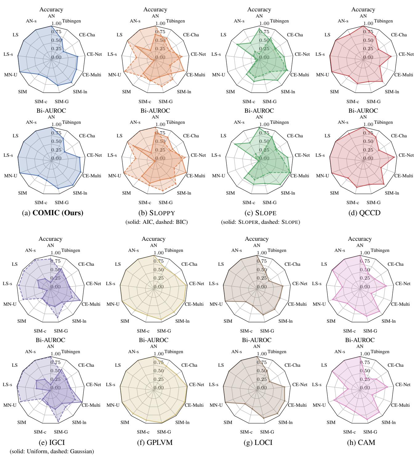
Interpreting the Radar Charts (Figure 1):

• Each spoke represents a different dataset (AN, LS, MN-U are synthetic; Tübingen is real).
• The farther out the colored polygon reaches, the better the performance.
• Panel (a) is COMIC. Notice how “full” the polygon is. It hits high accuracy across almost all datasets.
• Compare this to Panel (h) CAM. CAM performs well on “AN” (Additive Noise) datasets because it is designed for them. But look at “CE-Multi” or “Tübingen”—it collapses. It’s too rigid.
• Compare to Panel (d) QCCD. It performs well but struggles on the complex “CE-Multi” dataset compared to COMIC.

Overall Aggregated Results:

The bar chart below summarizes the average performance across all datasets.

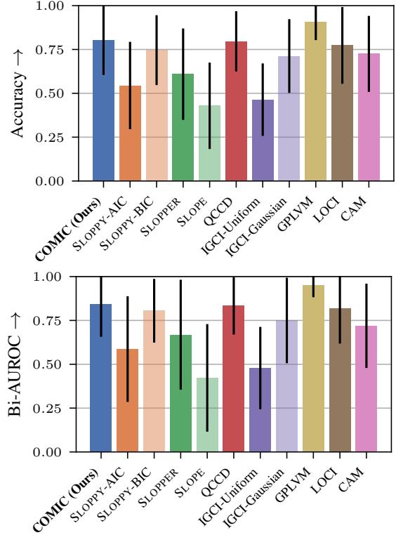
Key Takeaways from the Data:

1. COMIC vs. Maximum Likelihood (LOCI/CAM): COMIC outperforms the maximum likelihood methods (green/orange bars on the bottom right). This validates the hypothesis: fitting the data well isn’t enough; you must penalize complexity. Maximum likelihood methods overfit the “wrong” direction, making it look plausible.
2. COMIC vs. GPLVM: The Gaussian Process method (GPLVM) is the only competitor that matches or slightly edges out COMIC in some metrics. However, the authors note a crucial practical difference: GPLVM is computationally heavy, requiring GPUs and significant time. COMIC, using efficient Neural Network backpropagation, balances performance with scalability.
3. Real-World Performance: On the Tübingen dataset (real data), COMIC achieved comparable or better accuracy than most complexity-based methods. This is critical because real-world data rarely follows the clean mathematical rules of synthetic data.

Robustness

The authors also ran “ablation studies” (tests to see which parts of the model matter).

• Network Width: They found that if the neural network is too wide (e.g., 200 hidden neurons for a simple variable pair), the variational inference starts to ignore the data (the posterior collapses to the prior). A moderate width (10-50 neurons) worked best.
• Priors: Using a Uniform hyperprior for the variance of the weights worked better than simpler fixed priors.

Conclusion & Implications

The paper “Identifying Causal Direction via Variational Bayesian Compression” offers a compelling new tool for the causal discovery toolbox.

By equating causality with compressibility, the authors leverage the immense power of modern Deep Learning to solve a problem that has plagued statisticians for a century. The method, COMIC, treats the description length of a Neural Network as a proxy for the complexity of nature’s mechanisms.

Why does this matter?

1. Flexibility: unlike previous methods that assumed linear relationships or specific noise types, COMIC uses Neural Networks, allowing it to adapt to complex, non-linear, heteroscedastic relationships found in biology and finance.
2. Principled Complexity: It solves the “black box” problem of Neural Networks in this context. We aren’t just looking at test error; we are measuring the information content of the network itself via Variational Inference.
3. Scalability: It offers a path toward causal discovery that is more scalable than Gaussian Processes.

While the current version focuses on bivariate cases (just two variables), the authors suggest that the underlying principle—Variational Bayesian compression—could be extended to multivariate networks. This opens the door to discovering complex causal graphs in large systems, potentially helping us disentangle complex webs of cause and effect in fields ranging from genomics to climate science.

In the search for the arrow of time, it turns out that the best map might just be the one that takes up the least amount of space.