Introduction

Imagine two clouds of points floating in a 2D plane: one cloud is red, the other is blue. Your task is to pair every red point with a blue point such that the sum of the distances between the paired points is minimized. This is the Euclidean Bi-Chromatic Matching problem.

While this sounds like a pure geometry puzzle, it is actually the computational backbone of the 1-Wasserstein distance (also known as the Earth Mover’s Distance). This metric is ubiquitous in modern computer science, used for everything from comparing probability distributions in Machine Learning (like in WGANs) to analyzing drift in time-series data and comparing images in Computer Vision.

Historically, we have good algorithms for solving this in a static setting—where the points don’t move. But what if the data is alive? What if points are constantly appearing and disappearing? In this dynamic setting, re-running a static algorithm after every change is excruciatingly slow. Until now, the best dynamic approaches still required linear time—\(O(n)\)—to handle a single update. If you have millions of data points, that is simply too long to wait.

In a recent paper, researchers presented a massive leap forward: the first fully dynamic algorithm with sub-linear update time. Specifically, for any small parameter \(\varepsilon\), their method handles updates in \(O(n^\varepsilon)\) time while maintaining a solution that is an \(O(1/\varepsilon)\)-approximation of the optimal matching.

In this post, we will tear down this complex algorithm to understand how it achieves such speed. We will look at how it uses grid-based hierarchies, how it “implicitly” moves points around, and how it avoids redoing work when the data changes.

The Problem: Measuring Distance Between Distributions

Before diving into the solution, let’s formalize the problem. We are given a set \(A\) (red points) and a set \(B\) (blue points) in \(\mathbb{R}^2\). We assume \(|A| = |B| = n\). We want to find a bijection (a perfect matching) \(\mu: A \rightarrow B\) that minimizes the total Euclidean distance.

This problem is equivalent to computing the 1-Wasserstein distance between two discrete measures, defined formally as:

In a dynamic scenario, we receive a stream of updates. An update might insert a new red point and a new blue point, or delete an existing pair. Our goal is to maintain a valid matching with a low total cost, without having to calculate the whole thing from scratch every time.

The Core Method

The researchers’ approach is built on a “divide and conquer” strategy using spatial decomposition. However, they twist standard techniques in two clever ways: they use a bottom-up construction (building from small cells to large ones) and they use implicit matchings to handle data without iterating through every single point.

1. The Hierarchical Grid (The p-tree)

The foundation of the algorithm is a data structure called a restricted p-tree. Think of this as a Quadtree on steroids.

In a standard Quadtree, a square cell is divided into 4 smaller squares. In a p-tree, a cell of side length \(L\) is divided into a grid of \(p \times p\) subcells (where \(p\) is a parameter, usually a power of 2 like \(n^\varepsilon\)). This increases the branching factor, making the tree shallower, which is crucial for speed.

The algorithm randomly shifts the entire coordinate system at the start. This is a standard trick in geometric algorithms to ensure that, with high probability, short edges in the optimal matching don’t get “cut” by the boundaries of the large grid cells.

2. Bottom-Up Matching and “Excess”

The algorithm builds the matching starting from the leaves (the smallest grid cells) up to the root. Here is the intuition for a single node \(v\) in the tree:

1. Local Matching: Look at all the red and blue points strictly inside this cell.
2. Greedy Pairing: If the cell contains, say, 10 red points and 8 blue points, we know we can match 8 pairs immediately within this cell. We don’t know exactly which ones yet, but we know 8 blues will cancel out 8 reds.
3. Forwarding Excess: The remaining 2 red points cannot be matched here. They are the “excess.” We pass these 2 red points up to the parent node. The parent will try to match them with excess blue points coming from a different child cell.

This process ensures that points are matched as locally as possible. Short edges are prioritized because points are only sent to the parent (which represents a larger spatial area) if they absolutely cannot find a partner in their current, smaller neighborhood.

3. Implicit Matchings: The Key to Speed

If we explicitly stored and processed every point at every level of the tree, the algorithm would be slow. The “excess” sets passed to the root could be size \(O(n)\), leading to linear time complexity.

The researchers solve this by using Implicit Matchings.

Instead of passing the exact coordinates of the excess points to the parent, the algorithm aggregates them. If a child cell has excess red points, the parent views them as being located at the center of that child cell.

Inside a parent node \(v\), we have a grid of sub-cells. Some sub-cells have excess red points, and some have excess blue points. The algorithm solves a Geometric Transportation Problem (a generalized matching problem) between the centers of these sub-cells.

Let’s visualize this using a figure from the paper:

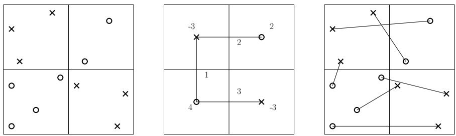
• Left Image: The actual input points in a grid.
• Middle Image: The Implicit Matching. The points are “snapped” to the center of their cells. The numbers represent supply (red) and demand (blue). The edges show how much “flow” (matching mass) moves between cell centers. This is much faster to compute because there are only \(p^2\) cell centers, regardless of how many actual points are inside.
• Right Image: The Explicit Matching. The flow between centers is translated back into specific edges between the real points.

By solving the problem on the “aggregated” instance (Middle), the algorithm gets a solution that is very close to the cost of the optimal matching on the real points, but it computes it in time depending on \(p\) (the grid size), not \(n\) (the total points).

4. Going Dynamic

So, how does this structure handle an update in sub-linear time?

When a new point \(x\) is inserted:

1. Leaf Update: The point falls into exactly one leaf cell. The local matching at that leaf might change.
2. Path to Root: This change might create a new “excess” point that gets passed to the parent. The parent updates its implicit matching (the transportation problem between cell centers). This might change the excess passed to its parent, and so on.
3. Limited Scope: Crucially, this chain reaction only travels up the path from the leaf to the root. Since the tree is shallow (depth roughly \(1/\varepsilon\)) and the work at each node depends on \(p\) (which is \(n^\varepsilon\)), the total update time is roughly \(O(n^\varepsilon)\).

The algorithm doesn’t need to look at the whole dataset. It only repairs the “damage” caused by the new point along a single branch of the tree.

The Approximation Guarantee

You might wonder: by snapping points to grid centers and matching them greedily, don’t we lose accuracy?

Yes, strictly speaking, this is an approximation algorithm. We sacrifice exactness for speed. However, the researchers prove that the error is bounded. Specifically, the expected cost of the matching \(\mu_a\) produced by the algorithm is related to the optimal cost \(c(\mu^*)\) by:

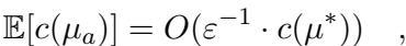
This equation states that the cost is at most \(O(1/\varepsilon)\) times the optimal cost. If you want a tighter approximation (smaller \(\varepsilon\)), the tree becomes deeper and the grid finer, which increases the runtime. This is a classic trade-off.

Experiments and Results

The theory is sound, but how does it perform in practice? The authors tested their implementation against standard baselines using synthetic data (Uniform, Gaussian) and real-world data (NYC Taxi trips).

Speedup vs. Static Algorithms

The primary motivation for this work is speed. The graph below shows the “speedup factor”—how much faster the dynamic algorithm is compared to re-running a static approximation from scratch.

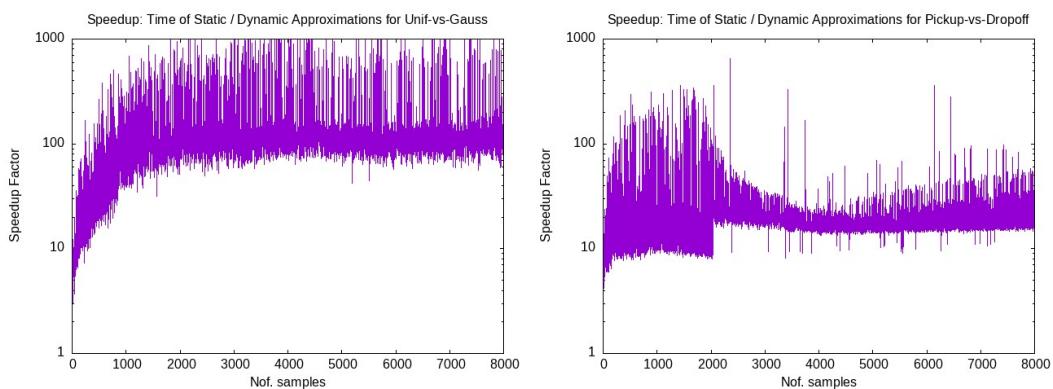
The results are stark. The dynamic algorithm is orders of magnitude faster (note the log scale). As the dataset size grows (x-axis), the gap widens. For applications requiring real-time response, a static re-computation simply isn’t feasible.

Convergence and Scalability

It is also important to verify that the algorithm actually converges to the correct Wasserstein distance as sample sizes increase, and that the update times remain low.

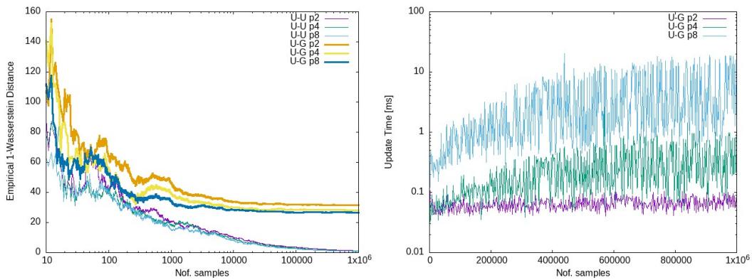
• Left Plot: Shows the estimated Wasserstein distance. Notice how the approximation curves (purple, cyan, green) track the curve of the exact solution.
• Right Plot: Shows the update time in nanoseconds/milliseconds. Even as the number of samples grows to \(10^6\), the update time remains incredibly low (often in the microsecond or millisecond range), confirming the sub-linear behavior.

Real-World Application: Taxi Data

To simulate a real-world scenario, the researchers used NYC Taxi data, treating pickup locations as red points and drop-off locations as blue points. They used a sliding window to simulate points entering and leaving the system.

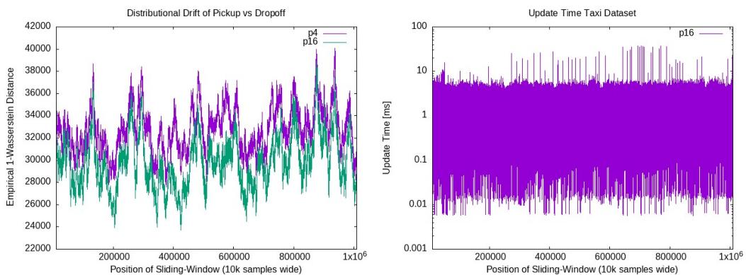
The Left Plot shows the algorithm tracking the “drift” (change in distribution) over time. The estimated distance fluctuates as the city’s traffic patterns change. The Right Plot shows the update time remaining stable and low throughout the simulation. This proves the algorithm’s viability for monitoring live data streams.

Accuracy Comparison

Finally, let’s look at how close the approximation gets to the exact solution.

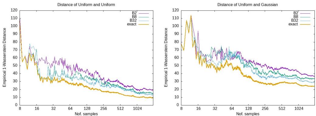
Here, the orange line is the exact solution. The other lines are approximations with different grid parameters (\(p\)). While there is a gap, the approximations follow the exact trend perfectly. In many machine learning applications (like training GANs), the gradient or the trend of the distance is more important than the exact numerical value, making these approximations highly effective.

Conclusion

The “Fully Dynamic Euclidean Bi-Chromatic Matching” paper represents a significant algorithmic advance. By moving from linear-time updates to sub-linear time \(O(n^\varepsilon)\), it opens the door for real-time applications that were previously impossible.

The core innovations—nested grids, bottom-up greedy matching, and implicit representation via transportation problems—allow the algorithm to ignore the vast majority of the dataset during an update, focusing only on the specific spatial regions affected by the change.

For students and practitioners in geometric optimization, this paper is a perfect example of how relaxing the requirement for an “exact” solution allows for massive gains in performance, provided you can bound the error. As datasets continue to grow into the millions and billions, these sub-linear dynamic algorithms will likely become the standard for handling geometric data in motion.