](https://deep-paper.org/en/paper/2505.14170/images/cover.png)
Introduction
In the world of machine learning, data is often neat and tabular. But in the real world—especially in biology, chemistry, and social sciences—data is messy and interconnected. It comes in the form of graphs: molecules are atoms connected by bonds; social networks are people connected by friendships.
To make sense of this data, we use Graph Convolutional Networks (GCNs). These powerful neural networks can predict properties like whether a molecule is soluble in water or which social group a user belongs to. We call this task Graph Property Learning.
But there is a catch. GCNs are notoriously expensive to train. As graph datasets grow into the millions (think of e-commerce networks or massive chemical databases), the computational cost of training these models skyrockets. We need a way to make them learn faster without sacrificing accuracy.
This brings us to a fascinating new research paper: “Nonparametric Teaching for Graph Property Learners.”
The researchers propose a new paradigm called GraNT (Graph Neural Teaching). Instead of feeding data randomly to the GCN, they introduce a “teacher” that strategically selects the most informative examples. By bridging the gap between deep learning on graphs and the theoretical framework of Nonparametric Teaching, they achieve a reduction in training time of over 30-40%.
In this post, we will walk through the problem, the heavy-lifting theory behind the solution, and the impressive results.
The Problem: The Cost of Implicit Mapping
At its core, inferring the property of a graph involves learning a mapping. You feed a graph \(G\) into a function, and it spits out a property \(y\).
In traditional mathematics, we might have a formula. In deep learning, this mapping is implicit. We don’t know the formula; we are trying to approximate it using a neural network (the GCN).
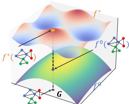
As shown in Figure 1, imagine the true relationship between a molecule’s structure and its energy state is the surface \(f^*\). Our GCN starts as a rough approximation, \(f^0\). The goal of training is to warp \(f^0\) until it matches \(f^*\).
The standard way to do this is Stochastic Gradient Descent (SGD): you pick a batch of graphs, check the error, update the weights, and repeat. But not all graphs are equally useful at all stages of training. Some are “easy” and don’t teach the model much; others are “hard” and drive significant updates. Random sampling ignores this, leading to wasted computational cycles.
Machine Teaching is the field dedicated to fixing this. It asks: Is there an optimal set of examples (a teaching set) that can guide the learner to the target function faster than random selection?
While Machine Teaching has existed for a while, it usually assumes the target function is simple (parametric). This paper applies Nonparametric Teaching—which deals with complex, function-space mappings—to the world of Graph Neural Networks.
The Theoretical Bridge
To apply teaching theories to GCNs, the authors had to solve a disconnect.
- GCNs update their parameters (weights) using gradient descent.
- Nonparametric Teaching updates the function itself in a mathematical space called a Reproducing Kernel Hilbert Space (RKHS).
To make GraNT work, the authors had to prove that training a GCN via parameters is mathematically consistent with teaching a nonparametric learner in function space.
1. Structure-Aware Updates
First, let’s look at how a GCN updates. Unlike a standard neural network (MLP) that treats input features independently, a GCN uses an adjacency matrix \(A\) to aggregate features from neighbors.
The authors analyzed a “Flexible GCN.” In this architecture, features are aggregated at different “hops” (neighbors, neighbors of neighbors, etc.) and concatenated.
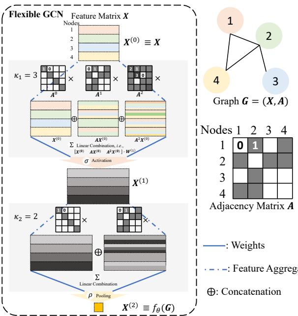
Figure 2 shows this flow. The input features \(X\) are multiplied by powers of the adjacency matrix (\(A^0, A^1, A^2...\)) to capture structural information. These are combined, passed through an activation function (\(\sigma\)), and pooled (\(\rho\)) to get the final output.
When we calculate the gradient to update the weights, the adjacency matrix \(A\) is baked into the math. The authors derived the explicit gradient and found that parameter updates are structure-aware. The gradient direction depends heavily on the graph’s topology, not just the node features.
2. The Dynamic Graph Neural Tangent Kernel (GNTK)
Here is the most complex and critical part of the paper. To connect the parameter updates to function space, the authors utilized the concept of the Neural Tangent Kernel (NTK).
In simple terms, the NTK describes how a neural network evolves during training. If you treat the network as a function \(f\), the change in that function over time can be described using a kernel \(K\).
For graphs, this is the Graph Neural Tangent Kernel (GNTK).

Figure 5 visualizes the computation of this kernel. It essentially measures the similarity between two graphs (\(G\) and \(G'\)) from the perspective of the neural network’s gradients. It involves taking the dot product of the gradients of the output with respect to the weights.
The authors proved a pivotal theorem (Theorem 5 in the paper):
The Dynamic GNTK, derived from gradient descent on the GCN parameters, converges to the structure-aware canonical kernel used in nonparametric teaching.
\[ \operatorname* { l i m } _ { t \infty } K _ { \theta ^ { t } } ( \pmb { G } _ { i } , \cdot ) = K ( \pmb { G } _ { i } , \cdot ) , \forall i \in \mathbb { N } _ { N } . \]
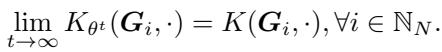
Why does this matter? This proof is the “license” to use Nonparametric Teaching algorithms on GCNs. It confirms that evolving the GCN via standard backpropagation is mathematically equivalent (in the limit) to performing functional gradient descent in the ideal teaching space. Because they behave the same way, we can use the “greedy selection” strategies from teaching theory to speed up GCN training.
The Solution: The GraNT Algorithm
With the theory established, the researchers proposed GraNT (Graph Neural Teaching).
The strategy is surprisingly intuitive. If the GCN update is equivalent to a functional gradient update, we want to maximize that gradient to converge as fast as possible.
Mathematically, maximizing the gradient update is roughly equivalent to selecting the data points where the current error is the largest.
The Algorithm
Instead of training on random batches, the “Teacher” selects specific graphs from the dataset to feed the “Learner” (GCN).
- Calculate Discrepancy: For a pool of candidate graphs, calculate the difference between the GCN’s current prediction \(f_{\theta}(G)\) and the true property \(f^*(G)\).
- Greedy Selection: Select the \(m\) graphs with the largest discrepancy.
- Update: Train the GCN on these \(m\) “hard” graphs.
- Repeat: Do this iteratively.
The selection criteria looks like this:
\[ \left\{ { { G } _ { i } } \right\} _ { m } ^ { * } = \underset { \left\{ { { G } _ { i } } \right\} _ { m } \subseteq \left\{ { { G } _ { i } } \right\} _ { N } } { \arg \operatorname* { m a x } } \left\| \left[ { { f } _ { \theta ^ { t } } } \left( { { G } _ { i } } \right) - f ^ { * } ( { { G } _ { i } } ) \right] _ { m } \right\| _ { 2 } . \]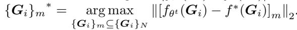
Two Flavors of GraNT
The authors proposed two variations to handle batch processing efficiently:
- GraNT (B) - Batch Level: The teacher looks at existing batches and picks the batches that have the highest average error. This is computationally cheaper because you don’t have to reshuffle data.
- GraNT (S) - Sample Level: The teacher looks at individual graphs, picks the hardest ones, and reorganizes them into new batches. This is more precise but slightly more computationally intensive.
Curriculum Learning: Notice that constantly feeding the model the hardest examples might be overwhelming at the start. The authors used a curriculum strategy: at the beginning, the teacher selects smaller subsets frequently (to help the model “digest”), and as training progresses, the selection interval widens.
Experiments and Results
Does this theoretical framework actually result in faster training? The authors tested GraNT on several benchmark datasets, including QM9 and ZINC (molecular property regression) and ogbg-molhiv (classification).
The results were compared against a standard training loop (“without GraNT”).
Graph-Level Tasks (Molecules)
The primary metric here is Wallclock Time versus Validation Loss/Error. We want the curve to drop to the bottom-left corner as fast as possible.
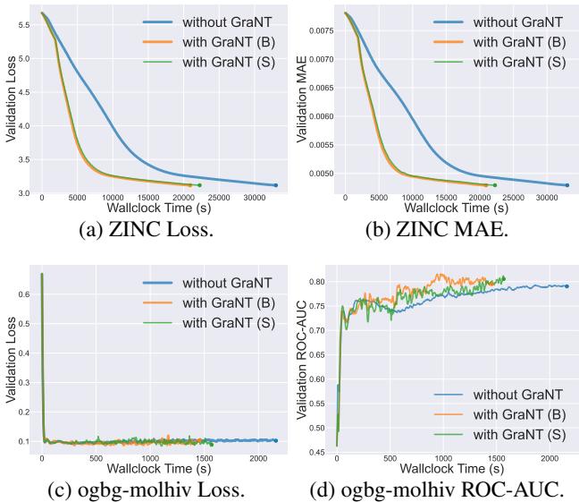
Figure 3 tells a compelling story:
- Charts (a) and (b) show the ZINC dataset. The Blue line (Without GraNT) is lazy; it takes a long time to reduce the error. The Orange (GraNT B) and Green (GraNT S) lines drop significantly faster.
- Charts (c) and (d) show the ogbg-molhiv classification task. GraNT reaches higher ROC-AUC scores (accuracy) much earlier than the baseline.
In terms of raw time, the savings are substantial.
- ZINC: Training time reduced by 36.62%.
- ogbg-molhiv: Training time reduced by 38.19%.
Node-Level Tasks
The method isn’t limited to classifying whole graphs. It also works for classifying specific nodes within a graph. The authors used synthetic datasets (gen-reg and gen-cls) to test this.
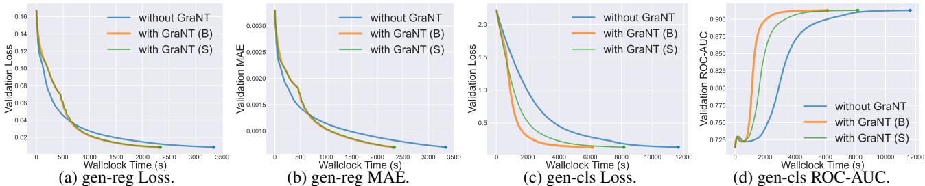
Figure 4 shows even more dramatic results. Look at Chart (c) (Loss) and Chart (d) (ROC-AUC). The GraNT curves (Orange/Green) skyrocket to high accuracy almost immediately, while standard training (Blue) lags behind significantly.
- Node-level Classification: Training time reduced by 47.30%.
Summary of Results
The table below summarizes the efficiency gains across different datasets. The key takeaway is that GraNT consistently reduces training time (often by a third or more) without hurting the final test performance (the error/accuracy metrics are comparable or better).
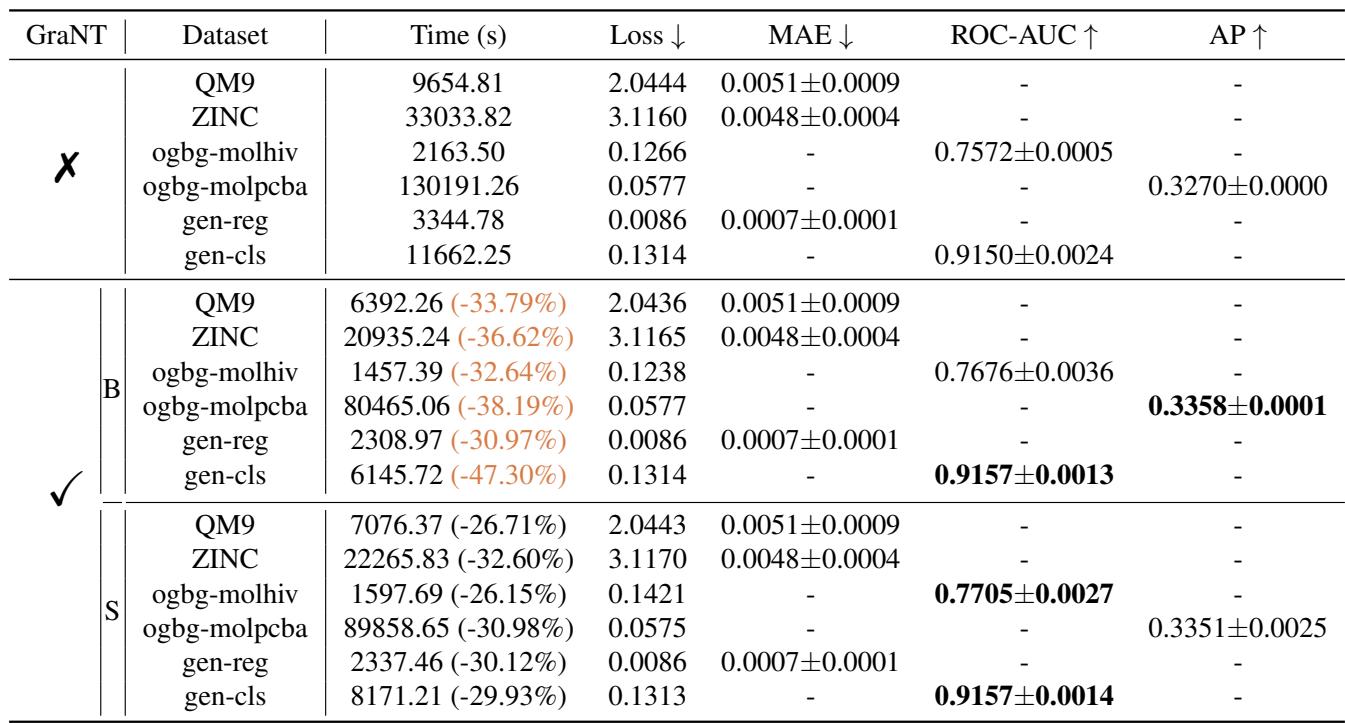
Both variants, GraNT (B) and GraNT (S), perform similarly. GraNT (B) is generally preferred because it is simpler to implement with standard batch loaders, whereas GraNT (S) requires reshuffling data, which adds a slight overhead.
Conclusion and Implications
The paper “Nonparametric Teaching for Graph Property Learners” offers a sophisticated solution to a practical problem. By looking at Graph Convolutional Networks through the lens of Nonparametric Teaching theory, the authors bridged the gap between parameter-based learning and function-based teaching.
Key Takeaways:
- Theoretical Alignment: The evolution of a GCN during training mathematically aligns with nonparametric functional gradient descent, thanks to the properties of the Graph Neural Tangent Kernel.
- Greedy is Good: Because of this alignment, a greedy “teacher” that selects the examples with the highest current error is mathematically justified in accelerating convergence.
- Real-World Speed: This isn’t just theory. The GraNT algorithm delivers 30-47% reductions in training time on standard benchmarks.
Why does this matter for the future? As we apply AI to increasingly complex scientific domains—like discovering new antibiotics or mapping protein interactions—the graphs we work with will become massive. Techniques like GraNT, which make learning more data-efficient and time-efficient, will be essential for scaling these models from research experiments to real-world tools.
Instead of throwing more compute at the problem, GraNT shows us that we can just be smarter about how we teach our models.