Rewriting the Map: How History-Driven Targets Revolutionize Graph Sampling

Imagine you are an explorer dropped into a massive, labyrinthine city—like a social network with millions of users or the vast topology of the internet. You have a mission: you need to estimate the average income of the population, or perhaps find a hidden community of bots. You can’t see the whole map at once; you can only see the street you are on and the intersections leading to neighbors.

This is the classic problem of Graph Sampling. To solve it, we typically use Random Walks—virtual agents that hop from node to node. However, simple random walks are notoriously inefficient. They get stuck in “cul-de-sacs” (tightly knit communities) and waste time revisiting the same nodes over and over again.

In recent years, researchers developed a clever fix called the Self-Repellent Random Walk (SRRW). It forces the explorer to say, “I’ve been here before, I should go somewhere else.” While effective, SRRW is like hiking with a heavy backpack; the computational math required to decide the next step is so heavy that it slows the explorer down to a crawl.

In this post, we will deep dive into a new framework presented at ICML 2025 by researchers from NC State University: the History-Driven Target (HDT). This method keeps the “self-repellent” intelligence but removes the heavy backpack. Instead of calculating complex physics for every step, it simply changes the map the explorer uses, making highly efficient sampling possible on massive graphs.

The Problem: Getting Stuck in the Graph

Graph sampling is fundamental to network science. Whether it’s training AI on graph data, crawling the web, or analyzing blockchain transactions, we need to generate samples from a target distribution \(\mu\) (often a uniform distribution across all nodes).

The standard tool for this is Markov Chain Monte Carlo (MCMC). A “walker” sits at a node, picks a neighbor, and decides to move or stay based on a probability rule. The most famous version is the Metropolis-Hastings (MH) algorithm.

While theoretically sound, standard MH suffers from slow mixing. If the graph has “bottlenecks”—narrow bridges between large clusters—the walker tends to get trapped in one cluster for a long time before crossing the bridge. This leads to high variance in our estimates; we might think the whole world looks like Cluster A simply because we haven’t found the bridge to Cluster B yet.

The Previous Solution: SRRW

To fix this, researchers introduced the Self-Repellent Random Walk (SRRW). The intuition is simple: if you have visited Node A ten times and Node B only once, you should be much more likely to move to Node B next.

SRRW achieves this by modifying the Transition Kernel—the actual probability mechanics of moving from one state to another.

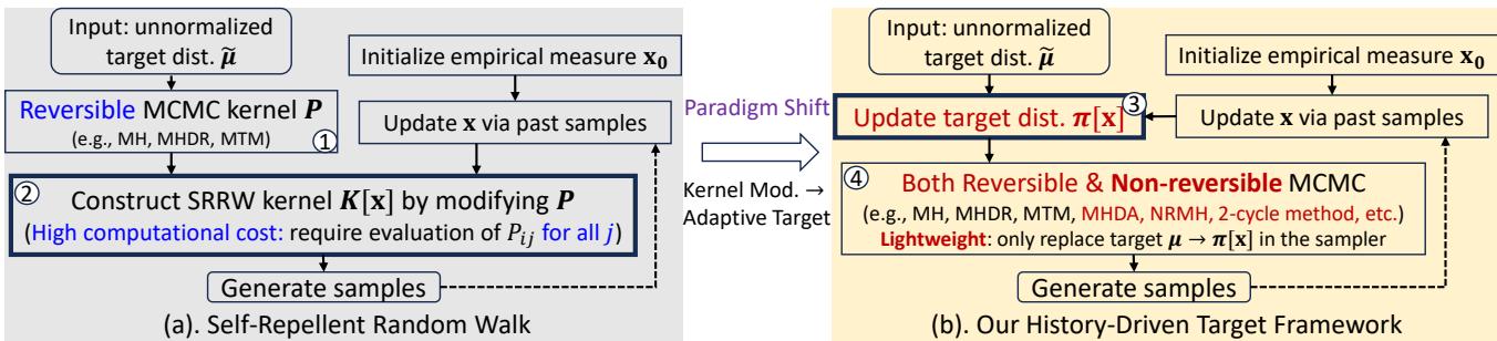
As shown in Figure 1 (a) above, the SRRW process involves taking the history of visits (\(\mathbf{x}\)), and using it to construct a new kernel \(K[\mathbf{x}]\). This kernel actively pushes the walker away from frequently visited states.

The math for the SRRW kernel looks like this:

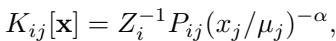
Here, \(x_j\) is the visit frequency and \(\mu_j\) is the target probability. The term \((x_j/\mu_j)^{-\alpha}\) creates the repulsion. If \(x_j\) is high (visited often), the probability of moving there drops.

The Flaw in SRRW: Look closely at the term \(Z_i^{-1}\) in the equation above. That is a normalizing constant. To calculate it, you must sum the probabilities of moving to every single neighbor of your current node \(i\).

If you are on a node with 5 neighbors, that’s fine. If you are on a “hub” node (like a celebrity on Twitter/X) with 100,000 neighbors, you must perform a massive calculation just to take one step. This computational overhead destroys the efficiency gains. Furthermore, SRRW strictly requires the underlying Markov chain to be “reversible,” ruling out many advanced, faster sampling techniques.

The Paradigm Shift: From Kernel to Target

The authors of the HDT paper asked a brilliant question: Why change the physics of the walk (the kernel) when we can just change the destination (the target)?

Instead of creating a complex new transition rule that forces the walker away from past states, the History-Driven Target (HDT) framework simply lies to the walker about the target distribution.

In standard MCMC, the walker tries to converge to a static target \(\mu\). In HDT, we replace \(\mu\) with a dynamic, history-dependent target \(\pi[\mathbf{x}]\).

Designing the New Target

The new target distribution \(\pi[\mathbf{x}]\) evolves over time. As the walker accumulates history (represented by the empirical measure \(\mathbf{x}\)), the target shifts to prioritize under-explored areas.

The formula for this new target is elegant and simple:

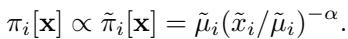
Let’s break this down:

• \(\tilde{\pi}_i[\mathbf{x}]\) is the unnormalized target probability for node \(i\).
• \(\tilde{\mu}_i\) is the original target (e.g., node degree or uniform value).
• \((\tilde{x}_i / \tilde{\mu}_i)^{-\alpha}\) is the feedback term.

If node \(i\) has been visited more than it “should” be (i.e., \(\tilde{x}_i\) is large relative to \(\tilde{\mu}_i\)), the term becomes small. The target probability \(\pi_i\) decreases. The MCMC sampler, simply doing its job of following the target, will naturally avoid this node because it now thinks the node is “unimportant.”

Conversely, if a node is under-visited, \(\pi_i\) increases, acting like a magnet pulling the walker toward unexplored regions.

Why This is a “Lightweight” Revolution

The genius of this approach lies in how it integrates with the Metropolis-Hastings (MH) algorithm. In MH, we accept a move from node \(i\) to node \(j\) based on an Acceptance Ratio.

Because the HDT framework modifies the target, not the kernel mechanics, the acceptance ratio becomes:

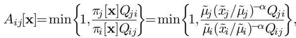
Notice something crucial here? There are no sums. There is no normalizing constant \(Z_i\) that requires checking all neighbors. We only need the values for the current node \(i\) and the proposed node \(j\).

This reduces the computational cost from \(O(\text{neighbors})\) in SRRW to \(O(1)\) in HDT. This is a massive speedup for dense graphs or high-dimensional problems.

The Algorithm: How It Runs

The HDT framework is designed to be a “plug-and-play” module. You can take any existing MCMC sampler (Base MCMC) and upgrade it with HDT.

Here is the flow of the algorithm:

1. Initialize the walker at a node and give every node a tiny “fake” visit count (to avoid division by zero).
2. Loop for \(T\) steps:

• Propose a new state using your base sampler (e.g., pick a random neighbor).
• Calculate the acceptance probability using the formula above (Image 009), which uses the current history \(\mathbf{x}\).
• Accept or Reject the move.
• Update History: Increment the visit count for the current node. This instantly updates the target \(\pi[\mathbf{x}]\) for the next step.

The history \(\mathbf{x}\) updates according to this stochastic approximation:

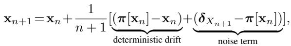
This equation shows that the history \(\mathbf{x}_{n+1}\) is a mixture of the old history \(\mathbf{x}_n\) and the new sample \(\delta_{X_{n+1}}\). This constant updating creates a feedback loop: as you visit a place, you make it less attractive, forcing you to move on.

Theoretical Guarantees: It Converges!

You might worry: “If we keep moving the goalposts (changing the target), will the walker ever actually map the true distribution \(\mu\)?”

The authors provide rigorous mathematical proofs to answer “Yes.”

1. Convergence (Ergodicity)

They prove that the empirical measure \(\mathbf{x}_n\) converges almost surely to the true target \(\mu\). The system can be modeled by a differential equation (ODE):

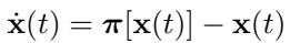
The system naturally drifts toward the equilibrium where \(\pi[\mathbf{x}] = \mathbf{x}\). The design of the target ensures that the only point where this happens is when \(\mathbf{x} = \mu\).

2. Variance Reduction (The “Zero Variance” Effect)

Standard random walks have variance related to the “spectral gap” of the graph. If the gap is small (bottlenecks), variance is huge.

HDT reduces this asymptotic variance significantly. The variance is scaled down by the “repellence parameter” \(\alpha\):

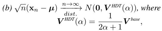
If you set \(\alpha=0\), you get the standard variance (\(V^{base}\)). As you increase \(\alpha\) (making the walker hate revisits more strongly), the variance \(V^{HDT}\) shrinks toward zero. This means you need fewer samples to get an accurate estimate.

3. The Cost-Based Advantage

This is the most critical theoretical contribution. SRRW also reduces variance, but it “pays” for it with expensive computation.

The authors derived a Cost-Based Central Limit Theorem. They compared the variance achievable per unit of computing budget (\(B\)).

This inequality states that the cost-adjusted variance of HDT is lower than SRRW by a factor roughly equal to the average neighborhood size (\(\mathbb{E}[|\mathcal{N}(i)|]\)).

In plain English: On a social network where the average person has 500 friends, HDT is roughly 250 times more efficient than SRRW.

Experimental Results

The theory sounds great, but does it work on real data? The researchers tested HDT on several real-world graphs, including Facebook social networks and Peer-to-Peer (Gnutella) networks.

Accuracy vs. Steps

They measured Total Variation Distance (TVD), which quantifies how far the sampled distribution is from the truth (0 is perfect).

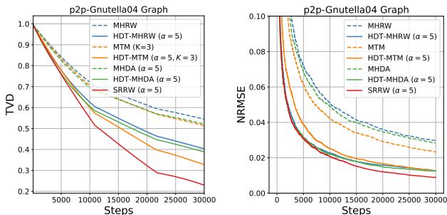
In Figure 2, look at the orange dotted line (HDT-MHRW). It drops much faster than the blue line (standard MHRW). This confirms that adding the history-driven target makes the sampler mix faster. Note that SRRW (solid blue line) also performs well in terms of steps, but remember—each of those steps was computationally expensive.

The Budget Showdown

When we compare accuracy against Computational Cost (time), the difference becomes stark.

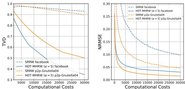
In Figure 3, look at the curves for the Facebook graph.

• SRRW (Blue dashed): drops slowly because it spends so much time calculating neighbor probabilities.
• HDT (Orange dotted): drops like a rock.

Because the Facebook graph is dense (high average degree), SRRW is penalized heavily. HDT achieves a low error rate almost immediately.

Flexibility: Non-Reversible Chains

One of the major limitations of the previous SRRW method was that it only worked with “Reversible” Markov chains (like standard Metropolis-Hastings). However, modern MCMC uses “Non-Reversible” chains (like MHDA or 2-cycle walks) because they inherently mix faster by avoiding backtracking.

Because HDT modifies the target and not the mechanics, it works seamlessly with non-reversible chains.

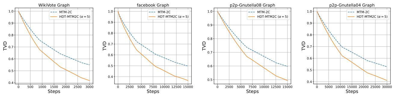
Figure 7 shows the “2-cycle” sampler (a non-reversible method). The solid orange line (HDT version) consistently outperforms the standard version (dashed blue). This proves HDT is a universal booster for graph sampling algorithms.

Scaling Up: The Memory Challenge

There is one catch. To run HDT, you need to track the history \(\mathbf{x}\) (visit counts) for every node. If your graph has 100 million nodes, storing a vector of size 100 million is memory-intensive.

The authors proposed a heuristic solution: Least Recently Used (LRU) Cache.

Instead of storing the history for every node, the algorithm only remembers the nodes it has visited recently. If the cache is full, it forgets the oldest visits. For nodes not in the cache, it estimates their visit frequency based on their neighbors in the cache.

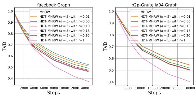
Figure 4 demonstrates the LRU performance.

• Even with a small cache (small \(r\)), the performance (orange/green lines) is significantly better than the standard Random Walk (starting at TVD 1.0).
• This suggests that local, recent history is the most important factor for self-repellence. You don’t need to remember what you did 10,000 steps ago to avoid getting stuck now.

Key Takeaways

The History-Driven Target (HDT) framework represents a significant step forward in MCMC sampling on graphs. By shifting the “self-repellent” mechanism from the transition kernel to the target distribution, the authors achieved the “holy grail” of sampling:

1. High Efficiency: Near-zero variance similar to previous state-of-the-art methods.
2. Low Cost: Updates are \(O(1)\) rather than \(O(\text{neighbors})\).
3. Universality: Works with almost any sampler (reversible or non-reversible).

For students and practitioners in data science, this highlights an important lesson: sometimes the best way to solve a complex pathfinding problem isn’t to build a smarter walker, but to simply draw a better map.

References

• Doshi et al., 2023. Self-repellent random walks on general graphs.
• Hu, Ma, & Eun, 2025. Beyond Self-Repellent Kernels: History-Driven Target Towards Efficient Nonlinear MCMC on General Graphs.