](https://deep-paper.org/en/paper/2505.19521/images/cover.png)
Imagine you are trying to walk through a crowded room in the dark. You can’t see perfectly; perhaps you only have a dim flashlight that flickers. You know roughly how your legs work (your dynamics), but your perception of where the furniture is (the environment) is noisy and uncertain. If you assume you know exactly where everything is, you will likely stub your toe. If you are too paralyzed by fear, you won’t move at all.
This scenario encapsulates one of the fundamental challenges in modern robotics: Learning unknown dynamics under environmental constraints with imperfect measurements.
In a recent paper, researchers Dongzhe Zheng and Wenjie Mei propose a sophisticated solution that bridges the gap between differential geometry and machine learning. Their work, Learning Dynamics under Environmental Constraints via Measurement-Induced Bundle Structures, introduces a mathematical framework that doesn’t just treat sensor noise as an annoyance to be filtered out. Instead, it treats uncertainty as a geometric structure—specifically, a fiber bundle.
In this post, we will deconstruct this paper, exploring how unifying measurements, dynamics, and constraints into a single geometric framework allows robots to learn safely, even when their sensors are lying to them.
The Core Problem: The Disconnect Between Math and Reality
To understand why this paper is significant, we first need to look at how safety-critical control is typically handled.
The gold standard for ensuring a robot doesn’t crash is the Control Barrier Function (CBF). A CBF acts like a virtual force field. As a robot approaches an unsafe region (like a wall), the CBF grows in value, forcing the controller to steer away. However, classical CBFs usually assume the robot knows its state \(x\) perfectly.
In reality, robots rely on sensors. A drone uses LiDAR or cameras; a robotic arm uses torque sensors. These measurements, denoted as \(y\), are related to the state \(x\) via a measurement map \(h(x)\), plus some noise \(v\).
\[ \begin{array} { l } { { \dot { x } = f ( x , u ) + g ( x ) w , \quad x ( 0 ) = x _ { 0 } } } \\ { { \qquad y = h ( x ) + v } } \end{array} \]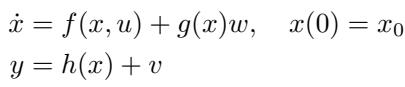
As shown in the equation above, the system evolves according to dynamics \(f(x, u)\) subject to disturbances \(w\), but we only observe \(y\).
Traditional approaches typically try to “clean” \(y\) to estimate \(x\) (using filters like Kalman filters) and then apply safety rules to that estimate. The authors argue that this separates the “sensing” problem from the “control” problem too much. By separating them, we lose the geometric relationship between the measurement uncertainty and the constraints. We need a framework where the uncertainty itself dictates the geometry of the safety maneuvers.
The Geometric Solution: Fiber Bundles
The authors’ key insight is that measurement uncertainty isn’t just probabilistic noise; it induces a geometric structure known as a Fiber Bundle.
What is a Fiber Bundle?
For those without a background in topology, a fiber bundle sounds intimidating, but the intuition is accessible. Imagine a field of wheat. The ground is the Base Space (the manifold \(\mathcal{M}\), representing the true states of the robot). Sticking up from every point on the ground is a stalk of wheat. This stalk is the Fiber.
In this framework, the “Total Space” \(\mathcal{E}\) is the combination of the state and the measurement space. For every true state \(x\), there is a set of possible measurements \(y\) that the sensors might report, constrained by the noise limits. This set of possible measurements forms the fiber above \(x\).
The authors define the fiber mathematically as:
\[ { { \pi } ^ { - 1 } } ( x ) = \left\{ ( x , y ) \in { \mathcal { E } } : y = h ( x ) + v , \| v \| \leq \delta _ { v } \right\} \]
Here, \(\pi^{-1}(x)\) represents the fiber at state \(x\). It contains all pairs of state and measurement \((x, y)\) where the measurement is within a bounded noise distance \(\delta_v\) of the true measurement map.
Why does this matter? By treating the system as moving through this “Total Space” (both state and measurement) rather than just the state space, the controller can naturally account for the fact that one true state could look like many different things to the sensors.
The Connection: Linking Dynamics and Measurements
In geometry, if you want to move from one fiber to another (i.e., how does the set of possible measurements change as the robot moves?), you need a mathematical object called a Connection.
The connection, denoted by \(\nabla\), dictates how the geometry “twists” as we move through the state space. It couples the dynamics of the state with the evolution of the measurements.
\[ \nabla _ { X } Y = \pi _ { * } ^ { - 1 } ( \nabla _ { \pi _ { * } X } ( \pi _ { * } Y ) ) + K ( x ) { \big ( } y - h ( x ) { \big ) } \]
In this equation, \(K(x)\) is a feedback gain operator. This is a dense mathematical way of saying that the system’s movement in the total space is a combination of the physical movement of the robot (the first term) and the “error” dynamics of the measurement (the second term). This structure allows the system to track how uncertainty propagates as the robot moves.
Propagation of Uncertainty
As the robot executes a trajectory, the noise in the process (\(w\)) and the noise in the measurement (\(v\)) interact. The differential relationships are captured here:
\[ \begin{array} { c } { { d \pi _ { * } ( X _ { f } ) = f ( x , u ) } } \\ { { d \pi _ { * } ( X _ { g } ) = g ( x ) w } } \\ { { d y = d h ( x ) + d v } } \end{array} \]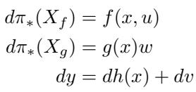
Because we are modeling this on the bundle, the uncertainty isn’t just a cloud of probability; it forms a geometric “tube” around the nominal trajectory.
\[ \mathcal { T } _ { \varepsilon } ( x , t ) = \{ y : d y ( y , h ( \phi _ { t } ( x ) ) ) \leq \varepsilon ( t ) \} \]
If the robot can keep its measurements inside this tube, it can maintain a probabilistic guarantee of safety. This geometric perspective allows the controller to be “measurement-aware.”
Measurement-Aware Control Barrier Functions (mCBFs)
Standard Control Barrier Functions say: “If \(h(x) \geq 0\), you are safe.” The authors introduce Measurement-Adapted Control Barrier Functions (mCBFs).
The core idea of an mCBF is that the safety margin should adapt based on the quality of the measurement. If the robot is in a state where sensors are noisy or the fiber is “large,” the safety function should become more conservative.
The definition of an mCBF requires three conditions:
\[ \begin{array} { l } { 1 . \mathrm { ~ } b ( x , y ) \geq 0 \implies x \in \mathcal { S } _ { 0 } } \\ { 2 . ~ \underset { u \in \mathcal { U } } { \operatorname* { i n f } } \left[ L _ { f } b + ( L _ { g } b ) w + \alpha ( b ) \right] \geq 0 } \\ { 3 . \left| b ( x , y _ { 1 } ) - b ( x , y _ { 2 } ) \right| \leq L _ { b } d y ( y _ { 1 } , y _ { 2 } ) } \end{array} \]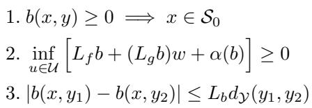
Let’s break these down:
- Safety Implication: If the barrier function \(b(x, y)\) is positive, the true state \(x\) must be in the safe set \(\mathcal{S}_0\).
- Forward Invariance: We must be able to find a control input \(u\) that keeps the barrier function positive (keeping us safe).
- Lipschitz Continuity (Crucial): The value of the safety function shouldn’t jump wildly if the measurement changes slightly. This condition bounds how much measurement noise can affect our safety perception.
The Adaptation Mechanism
How does the mCBF actually adapt? The authors propose a specific form for the barrier function:
\[ \begin{array} { c } { { \Phi ( x , y ) = \Phi _ { 0 } ( x , y ) - \alpha ( \| y - h ( x ) \| ) } } \\ { { { } } } \\ { { L _ { f } \Phi + ( L _ { g } \Phi ) w \geq - \beta ( \Phi ) \mathrm { a l o n g ~ s o l u t i o n s } } } \end{array} \]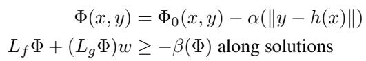
Notice the term \(-\alpha(\|y - h(x)\|)\). This subtracts from the safety margin as the deviation between the measurement \(y\) and the expected measurement \(h(x)\) grows.
- Good Sensing: \(y \approx h(x)\), the penalty is small, and the robot can act aggressively.
- Bad Sensing: \(y\) deviates from \(h(x)\), the penalty is large, and the safety boundary tightens effectively.
Probabilistic Safety Guarantees
Because noise is stochastic (random), guarantees are usually probabilistic. The framework proves that with these mCBFs, the probability of remaining safe is very high, bounded exponentially by the noise level.
\[ \mathbb { P } ( x ( t ) \in S _ { 0 } f o r a l l t \geq 0 ) \geq 1 - \exp ( - c / \delta _ { v } ^ { 2 } ) \]
This theorem states that the probability of staying in the safe set \(S_0\) depends on the measurement noise bound \(\delta_v\). As sensors get better (smaller \(\delta_v\)), safety approaches certainty.
Learning the Dynamics with Neural ODEs
So far, we’ve discussed geometry and safety. But the paper is also about learning. The robot doesn’t initially know its own dynamics function \(f(x, u)\).
The authors use Neural Ordinary Differential Equations (Neural ODEs) to approximate the dynamics. However, they don’t just throw a neural network at the raw data. They constrain the learning process using the bundle structure.
They define a learning operator \(\mathcal{L}\) that works on the bundle:
\[ \mathcal { L } ( \Phi ) ( x , y ) = \nabla \varepsilon \Phi ( x , y ) + \lambda R ( x , y ) \]
The update laws for the learned dynamics \(\hat{f}\) and the barrier function \(\Phi\) are driven by these operators:
\[ \begin{array} { l } { \dot { \hat { f } } = - \mathcal { L } _ { 1 } ( \hat { f } - f ) } \\ { \dot { \Phi } = - \mathcal { L } _ { 2 } ( \Phi - \Phi ^ { * } ) } \end{array} \]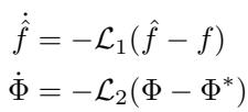
By embedding the learning process inside the geometric framework, the neural network is forced to respect the physical structure of the system (like symmetries in rotation or translation) and the measurement constraints.
The actual training loss function combines the dynamics error with an uncertainty-weighted norm:
\[ \begin{array} { c } { \displaystyle \dot { \theta } = - \Lambda \nabla _ { \theta } \mathcal { T } ( \hat { f } _ { \theta } , \mathcal { D } ) } \\ { \displaystyle \mathcal { T } ( \hat { f } , \mathcal { D } ) = \sum _ { i = 1 } ^ { N } \| \hat { f } ( x _ { i } , u _ { i } ) - \dot { x } _ { i } \| _ { \Sigma _ { i } ^ { - 1 } } ^ { 2 } } \end{array} \]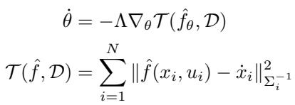
Here, \(\Sigma_i^{-1}\) weights the error. Data points with high uncertainty (noisy measurements) contribute less to the gradient update, preventing the neural network from “overfitting to noise.”
Experiments: Does it Work?
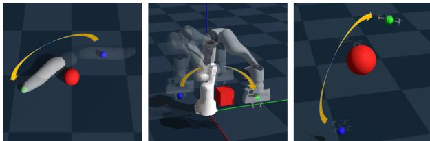
The theory is elegant, but robotics is an empirical science. The authors validated their framework on three distinct, challenging tasks using the Genesis physics engine.
The Experimental Setup
- Soft Worm Robot: A soft-body robot that moves via peristalsis. It has complex, non-linear dynamics and relies on visual sensors to avoid obstacles.
- Franka Emika Arm: A 7-degree-of-freedom robotic arm performing manipulation. It must avoid obstacles while reaching for objects, dealing with joint friction and payload variations.
- Quadrotor Drone: A flying drone navigating 3D space with aerodynamic disturbances and depth measurement noise.
Comparative Results
The authors compared their method (“Ours”) against several state-of-the-art baselines:
- Neural-CBF: Uses neural networks for barrier functions but without the bundle structure.
- GPMPC: Gaussian Process Model Predictive Control (a standard probabilistic method).
- SafetyNet & DataFilter: Other safe learning approaches.
The results, shown in the convergence plots below, are striking.
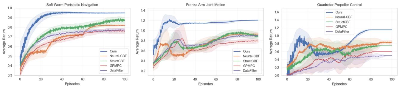
In all three tasks (Worm, Arm, Drone), the proposed method (blue line) converges to a higher return (better performance) significantly faster than the baselines. The shaded region represents the standard deviation—notice how the blue region is narrower? This implies the method is not only better but more consistent and stable.
Robustness to Noise
The true test of the “Measurement-Induced” framework is what happens when measurements get worse. The authors tested the success rate of the tasks under Low, Medium, and High noise levels (\(\sigma\)).
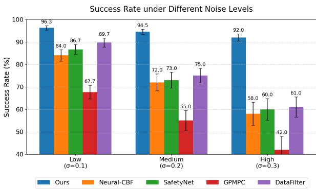
As shown in the bar chart:
- Low Noise (\(\sigma=0.1\)): Everyone does okay, but “Ours” is top (96.3%).
- High Noise (\(\sigma=0.3\)): This is where the geometric structure shines. Baseline methods like Neural-CBF crash to 58% success. GPMPC drops to 42%. The proposed method maintains a 92.0% success rate.
This confirms the hypothesis: by embedding the measurement uncertainty into the geometry of the controller (the bundle structure), the robot naturally becomes more conservative and robust when sensors degrade.
Detailed Metrics
The numerical results highlight the efficiency of the trajectories.
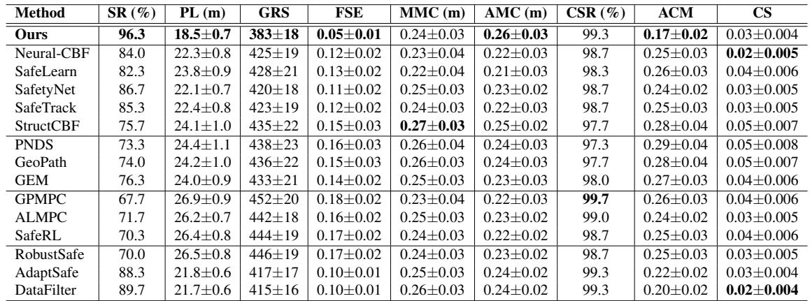
Looking at Table 1:
- Success Rate (SR): The proposed method achieves 96.3% on average, compared to 84% for Neural-CBF.
- Path Length (PL): The paths are shorter (18.5m vs 22.3m).
- Constraint Satisfaction (CSR): 99.3%.
Why are the paths shorter and safer? Traditional robust methods (like RobustSafe) achieve high safety by being overly conservative—they assume the worst case everywhere, leading to wide, inefficient paths. The Bundle Framework adapts. It is conservative only when necessary (high uncertainty) and efficient when measurements are clear.
Does the Bundle Structure Really Matter?
The authors performed an ablation study to see if the complex geometry was actually doing the heavy lifting. They removed the mCBF (safety) and the Bundle Structure to see what would happen.
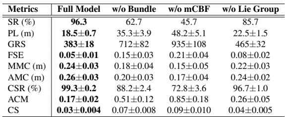
The results are damning for non-geometric approaches:
- w/o Bundle: Success rate drops from 96.3% to 62.7%. Path length nearly doubles.
- w/o mCBF: Success rate drops to 45.7%.
This proves that treating the state and measurement spaces as a unified fiber bundle is not just mathematical window dressing—it is the primary driver of the performance gains.
Convergence and Theory
Finally, the authors provide theoretical backing for their experimental success. They prove that the learned dynamics \(\hat{f}\) converge to the true dynamics \(f\) exponentially fast, with a residual error bounded by the measurement noise \(\delta_v\).
\[ \begin{array} { r } { \| \hat { f } - f \| _ { \varepsilon } \leq c _ { 1 } \exp ( - \lambda _ { 1 } t ) + c _ { 2 } \delta _ { v } } \\ { \mathbb { P } ( x ( t ) \in { \mathcal S } _ { 0 } ) \geq 1 - \exp ( - c _ { 3 } / \delta _ { v } ^ { 2 } ) } \end{array} \]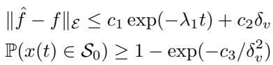
This gives us confidence that the neural network isn’t just memorizing trajectories, but is actually approximating the system dynamics accurately enough to maintain safety.
Conclusion
The paper Learning Dynamics under Environmental Constraints via Measurement-Induced Bundle Structures offers a compelling argument: Geometry matters.
In the quest for autonomous systems, it is tempting to rely solely on massive datasets and black-box neural networks. However, this work demonstrates that by respecting the underlying geometric structure of the problem—specifically, the relationship between where a robot is and what it sees—we can achieve significantly better results.
The Fiber Bundle framework allows for:
- Unified Modeling: Integrating dynamics, constraints, and sensor noise.
- Adaptive Safety: Safety margins that breathe with the uncertainty of the environment.
- Robust Learning: Neural ODEs that learn efficiently without overfitting to sensor noise.
For students of robotics and control theory, this represents a shift toward “embodied intelligence,” where the physical limitations of the agent (like its sensors) are central to how it learns to move, rather than afterthoughts to be filtered away.