Taming Chaos: How K²VAE Linearizes the Future for Accurate Time Series Forecasting

Predicting the future is one of the oldest human desires and one of the hardest mathematical challenges. In the realm of data science, this translates to Time Series Forecasting. While we have become quite good at predicting what happens in the next hour or day (short-term forecasting), predicting distant futures (long-term forecasting) remains a stumbling block.

The difficulty compounds when we move from point forecasting (predicting a single value, like “25°C”) to Probabilistic Time Series Forecasting (PTSF), where we try to predict a distribution (e.g., “25°C with a standard deviation of 2°C”). We need these probability distributions to make high-stakes decisions in energy grids, financial markets, and supply chains.

Today, we are diving deep into a new paper, K²VAE, which proposes a fascinating hybrid approach. It combines Koopman Operator Theory (from physics), Kalman Filtering (from control theory), and Variational AutoEncoders (from deep learning) to tackle the inherent chaos of long-term forecasting.

The Problem: Chaos and Error Accumulation

Why is Long-term Probabilistic Time Series Forecasting (LPTSF) so difficult?

1. Nonlinearity: Real-world systems (weather, traffic, stock prices) are nonlinear. They don’t follow straight lines; they loop, spike, and behave chaotically. Most statistical models struggle to capture these complex dynamics over long horizons.
2. Error Accumulation: If your model makes a tiny error at step 1, that error feeds into step 2, growing exponentially. By step 720, the prediction is often useless.
3. Inefficiency: Modern generative models, like Diffusion models, are great at distributions but are computationally heavy. They often require hundreds of iterative steps to generate a single prediction, making them slow and memory-hungry.

The researchers illustrate this problem vividly in the chart below.

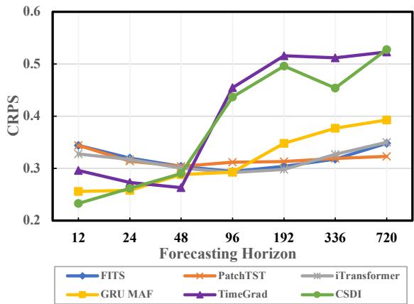
As shown in Figure 1, as the forecasting horizon extends (moving right on the x-axis), the error metric (CRPS, where lower is better) for standard probabilistic models explodes. In fact, point forecasting models (like PatchTST) often beat specialized probabilistic models simply because the probabilistic ones collapse under the weight of accumulated uncertainty.

The Core Idea: Linearizing the Nonlinear

The authors of K²VAE propose a clever workaround to the nonlinearity problem. Instead of trying to model the chaotic, nonlinear curve directly, what if we could transform the data into a different mathematical space where the behavior becomes linear?

This is the premise of Koopman Theory. If we can find the right measurement function, we can project a nonlinear system into a higher-dimensional space where its evolution is governed by a linear operator.

However, finding this perfect linear representation is difficult. The resulting linear system is often “biased” or imperfect. This is where the Kalman Filter comes in. The Kalman Filter is the gold standard for estimating the state of a linear system that has noise or errors.

K²VAE stands for Koopman-Kalman Variational AutoEncoder. The high-level workflow is:

1. KoopmanNet: Transforms the complex time series into a simplified linear system.
2. KalmanNet: Corrects that linear system and quantifies the uncertainty.
3. VAE: Generates the final probabilistic forecast based on the refined states.

Let’s look at the high-level data flow:

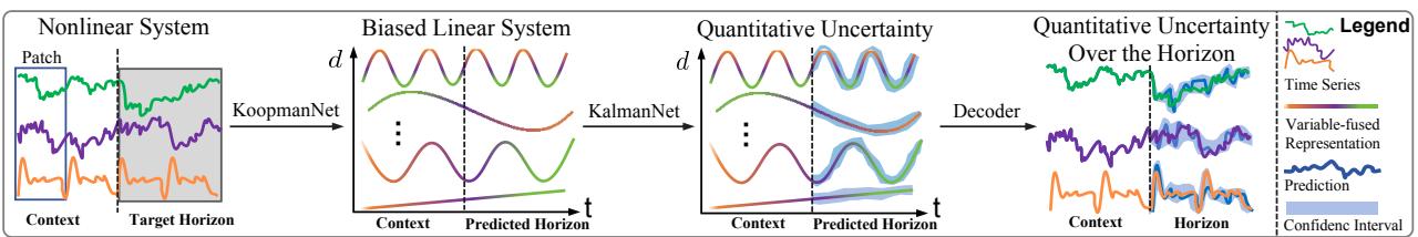
As seen in Figure 2, the model splits the task. The KoopmanNet creates a “Biased Linear System” (a rough linear sketch). The KalmanNet then takes this sketch, refines it, and—crucially—calculates the “Quantitative Uncertainty” (the confidence intervals). Finally, the Decoder maps everything back to real-world values.

Theoretical Foundations

Before dissecting the architecture, we need to briefly ground ourselves in the two “K"s of the name.

1. Koopman Theory

Koopman theory states that for a nonlinear dynamical system \(x_{k+1} = f(x_k)\), there exists an infinite-dimensional space of measurement functions \(\psi\) where the transition is linear.

Here, \(\mathcal{K}\) is the Koopman Operator. It allows us to step forward in time using simple matrix multiplication, which is computationally efficient and stable, provided we can learn the mapping \(\psi\).

2. Kalman Filter

The Kalman Filter is a recursive algorithm used to estimate the state of a linear system. It works in two beats:

1. Predict: Estimate the next state based on the current physics of the system.
2. Update: Look at the actual measurement, calculate the difference (residual), and adjust the prediction based on the Kalman Gain (how much we trust the model vs. the measurement).

In K²VAE, the Kalman Filter is implemented as a neural network layer (KalmanNet) to learn the optimal gains and covariance matrices from data.

The K²VAE Architecture

Now, let’s break down the model step-by-step.

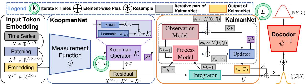
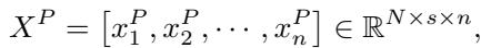
Step 1: Input Token Embedding

Time series data is often granular. To capture local semantic information, the model first uses a technique called patching. It breaks the time series into non-overlapping segments (patches), effectively treating time series segments like words in a sentence (tokens).

These patches are then projected into a high-dimensional embedding space. This allows the model to capture multivariate correlations (relationships between different variables, like temperature and electricity usage) implicitly.

Step 2: The KoopmanNet (Linearization)

The Encoder’s first job is to linearize the dynamics. It uses a neural network (MLP) as the measurement function \(\psi\) to project the embedded tokens into the “measurement space.”

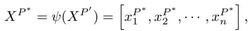
Once in this space, the model attempts to fit a linear transition matrix, the Koopman Operator \(\mathcal{K}\). The authors use a mix of a purely data-driven approach (using a technique called Extended Dynamic Mode Decomposition, or eDMD) and a learnable global operator.

By iterating this operator, the model generates a prediction of the future states.

Here, \(\hat{X}^C\) is the reconstructed context (past), and \(\hat{X}^H\) is the predicted horizon (future). Because the learned measurement function is never perfect, this linear system is biased. It captures the main trend but misses the nuances.

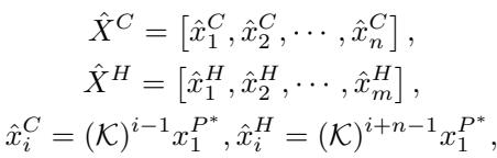
Step 3: Handling Residuals with the Integrator

To fix the bias, the model looks at what the Koopman linear system missed. It calculates the residual (the difference between the actual projection and the linear reconstruction).

An Integrator (based on a Transformer architecture) processes these nonlinear residuals.

The output \(U\) represents the nonlinear information that the simple linear operator couldn’t capture. This will serve as a “control input” for the Kalman Filter.

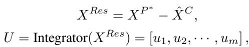
Step 4: The KalmanNet (Refinement & Uncertainty)

This is the heart of the innovation. The authors design a KalmanNet that treats the linear system from the KoopmanNet as an observation and the nonlinear residuals as a control force.

The KalmanNet maintains a state estimate \(z_k\) and, crucially, a covariance matrix \(P_k\). This matrix mathematically represents the model’s uncertainty—exactly what we need for probabilistic forecasting.

The Prediction Step: First, the KalmanNet predicts the next state and the next uncertainty covariance.

The Update Step: Then, it refines this prediction using the information from the KoopmanNet. It calculates the Kalman Gain \(K_k\), which decides how much to adjust the state.

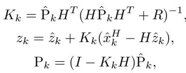
This step effectively fuses the linear trend (from Koopman) with the nonlinear adjustments (from the Integrator) while explicitly calculating the distribution of the data via \(P_k\).

Step 5: The Decoder (Generative Output)

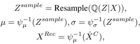
Finally, we need to get back to the original time series values. K²VAE uses the standard Variational AutoEncoder structure here. The KalmanNet gives us a refined state \(Z'\) and uncertainty \(P\). These define a variational distribution \(\mathbb{Q}(Z|X)\).

The model samples from this distribution and uses the inverse of the measurement function (\(\psi^{-1}\)) to decode the result back into the time series domain.

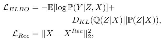
The training objective combines the Evidence Lower Bound (ELBO) from VAE theory with a reconstruction loss to ensure the linear system matches reality.

Why This Approach Wins: Efficiency & Accuracy

The K²VAE architecture offers a distinct advantage over diffusion-based models (like TimeGrad or TSDiff). Diffusion models generate data by iteratively “denoising” random noise, often requiring dozens or hundreds of passes through the network.

K²VAE, by contrast, relies on matrix multiplication (Koopman) and recursive updates (Kalman), which are computationally cheap.

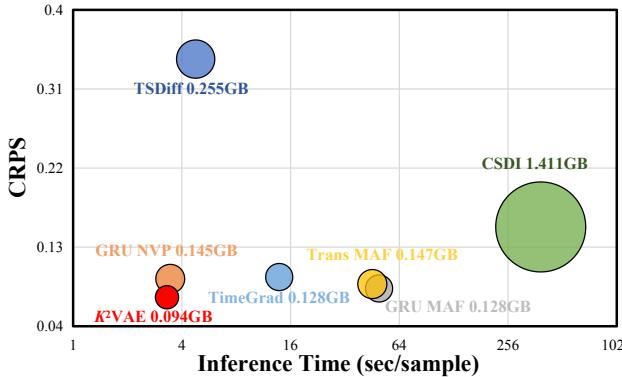
Figure 4 plots the Continuous Ranked Probability Score (CRPS, y-axis) against Inference Time (x-axis). Ideally, you want to be in the bottom-left corner (fast and accurate).

• CSDI (Green): Very accurate (high up on y-axis is actually bad CRPS, lower is better. Correction: The caption notes lower CRPS is better. CSDI has a CRPS of ~0.24, K2VAE is ~0.05). CSDI is accurate but extremely slow and memory-intensive.
• K²VAE (Red): sits in the bottom-left. It achieves the lowest error (CRPS ~0.05) while being roughly 10x-50x faster than the heavy generative models.

Experimental Results

The researchers tested K²VAE on widely used benchmarks (ETTh1, Electricity, Traffic, Weather) against the best models in the field.

Long-Term Forecasting Performance

The results for long-term forecasting (Predicting 720 hours ahead) are particularly impressive.

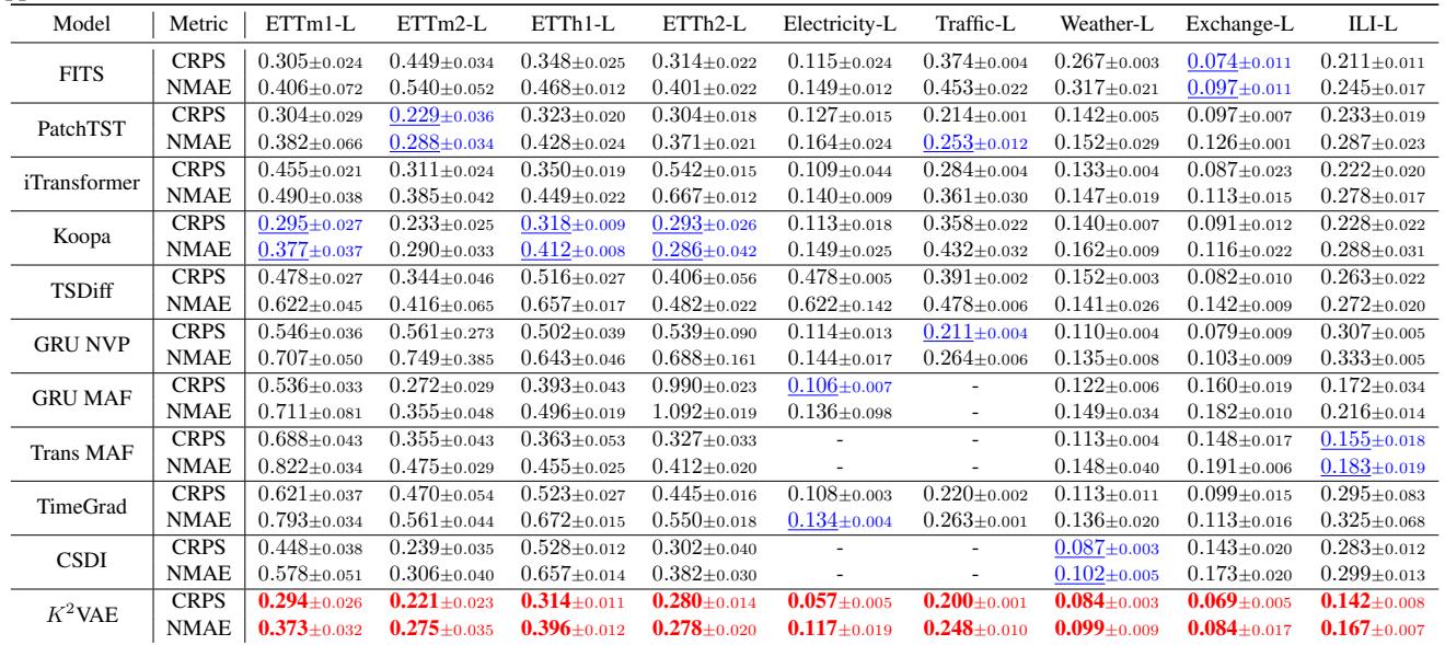
In Table 3, K²VAE (bottom row) consistently achieves the best (bold) or second-best (underlined) results across almost all datasets.

• On the Electricity-L dataset, K²VAE achieves a CRPS of 0.057, nearly half the error of the Transformer baseline (0.109).
• It significantly outperforms TimeGrad and CSDI, the previous state-of-the-art in probabilistic forecasting.

Visualizing the Uncertainty

Numbers are great, but in probabilistic forecasting, we want to see the confidence intervals. Does the model know when it is uncertain?

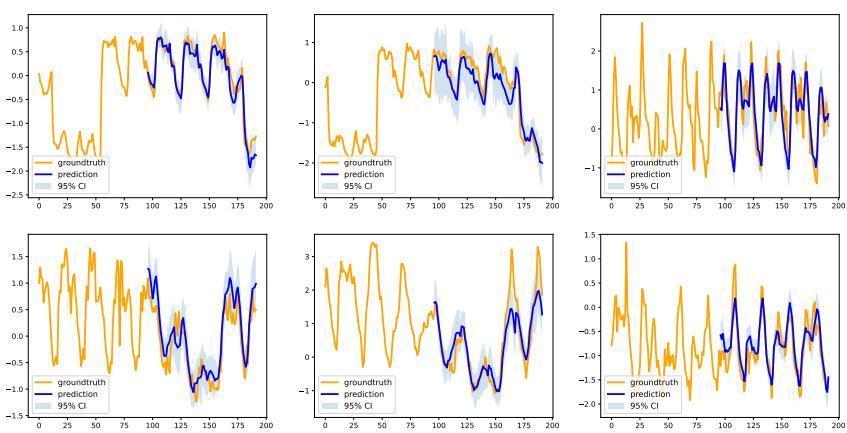
Figure 7 shows the forecasts on the Electricity dataset.

• Orange: Ground Truth.
• Blue Line: Prediction.
• Light Blue Shade: 95% Confidence Interval.

Notice how the confidence interval (the shaded region) tightly hugs the ground truth. Even when the series spikes or drops, the true value rarely falls outside the model’s predicted range. This reliability is crucial for applications like grid management, where underestimating the variance can lead to blackouts or overloaded transformers.

Short-Term Performance

While the model is designed for long-term tasks, it doesn’t sacrifice short-term accuracy.

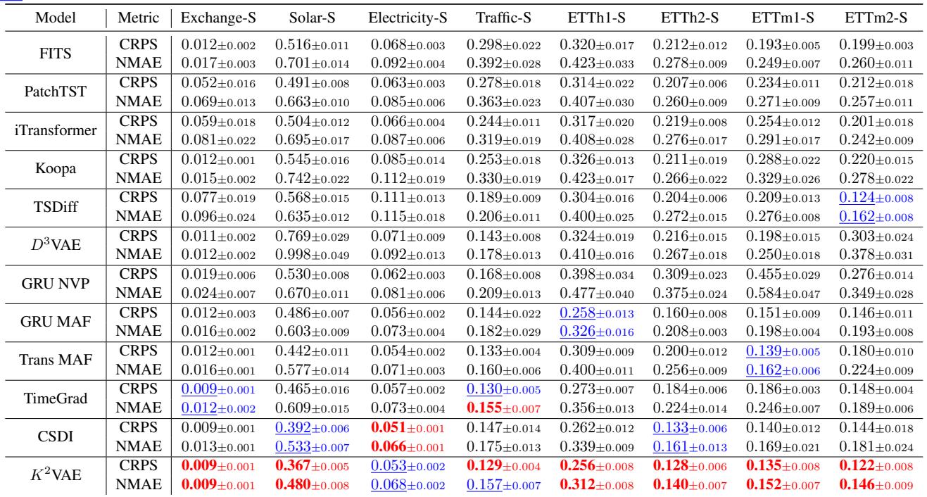
As shown in Table 2, K²VAE still outperforms specialized short-term models like PatchTST and TimeGrad on datasets like Solar and Traffic. This suggests that the “Linearization + Refinement” strategy is a robust way to model time series dynamics in general, regardless of the horizon length.

Key Takeaways

The K²VAE paper presents a compelling argument for moving away from purely “black box” deep learning toward “gray box” models that incorporate physical principles.

1. Divide and Conquer: Instead of forcing a neural network to learn complex nonlinear chaos directly, K²VAE splits the problem. It uses Koopman theory to find a linear simplification and Kalman filtering to handle the messy reality.
2. Explicit Uncertainty: By using the Kalman Filter’s covariance matrix naturally within a VAE, the model produces rigorous uncertainty estimates without the heavy computational cost of diffusion ensembles.
3. Speed Matters: In real-time decision-making systems (like high-frequency trading or real-time traffic control), you cannot wait seconds for a diffusion model to denoise a prediction. K²VAE’s efficiency makes it highly deployable.

For students and researchers in time series analysis, K²VAE demonstrates that the classical theories of the 20th century—Koopman (1931) and Kalman (1960)—are not obsolete. When supercharged with modern deep learning, they provide state-of-the-art solutions to our most complex prediction problems.