](https://deep-paper.org/en/paper/2505.23760/images/cover.png)
The open-source AI revolution has democratized access to powerful tools, from Large Language Models (LLMs) to text-to-image generators. However, this accessibility comes with a significant risk: malicious fine-tuning. A bad actor can take a safe, publicly available model and fine-tune it on a small dataset of harmful content—be it creating non-consensual deepfakes, generating hate speech, or designing malware.
This leads to a pressing safety question: Can we release a model that is “immune” to being taught bad behaviors, while still remaining useful for its intended purpose?
This concept is known as Model Immunization. Until recently, approaches to this were largely empirical—trial and error methods that seemed to work but lacked a solid theoretical foundation. In this post, we will dive deep into a research paper titled “Model Immunization from a Condition Number Perspective.” The authors propose a mathematically grounded framework that uses the condition number of the Hessian matrix to “lock” model parameters against harmful updates.
If you are a student familiar with gradient descent and basic linear algebra, you are about to see how these fundamental concepts can be weaponized for AI safety.
The Core Problem: Fine-Tuning as Optimization
To understand immunization, we first need to look at how a bad actor modifies a model. Typically, they perform transfer learning (specifically linear probing or fine-tuning). They take a pre-trained feature extractor, freeze most of it, and train a linear classifier on top using a harmful dataset \(\mathcal{D}_H\).
Mathematically, they are solving an optimization problem. They want to find weights \(\mathbf{w}\) that minimize a loss function \(\mathcal{L}\):
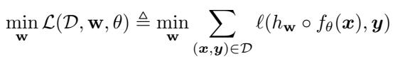
Here, \(f_\theta\) is the pre-trained feature extractor (parameterized by \(\theta\)) and \(h_\mathbf{w}\) is the classifier. The bad actor uses Gradient Descent to minimize this loss.
The Speed of Learning and the Condition Number
Here is the crux of the paper: Optimization is not always easy. The geometry of the loss landscape determines how quickly (or if) gradient descent converges to a solution.
If the loss landscape looks like a nice, round bowl, gradient descent zooms to the bottom. If it looks like a long, narrow valley, the optimizer bounces back and forth, converging very slowly.
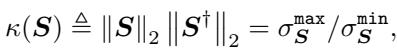
In linear algebra, this geometry is described by the Condition Number (\(\kappa\)) of the Hessian matrix (the matrix of second derivatives). The condition number of a matrix \(\mathbf{S}\) is defined as the ratio of its largest singular value to its smallest singular value:
Why does this matter? Because the convergence rate of steepest descent is bounded by this number. If \(\mathbf{w}^*\) is the optimal solution and \(\mathbf{w}_t\) is the weight at step \(t\), the distance to the solution decreases according to:
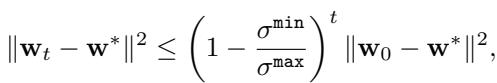
Look closely at that inequality. If the condition number \(\kappa = \sigma^{\max} / \sigma^{\min}\) is very large (a “ill-conditioned” problem), the term \((1 - \frac{\sigma^{\min}}{\sigma^{\max}})\) becomes very close to 1. This means the error shrinks tiny bit by tiny bit. Convergence takes forever.
The Immunization Insight: If we can force the condition number for the harmful task to be massive (infinity, ideally), the bad actor’s gradient descent will essentially stall. They won’t be able to fine-tune the model.
A Framework for Immunization
The authors define an “immunized” model based on three specific requirements involving the condition number. Let \(\theta^I\) be the parameters of our immunized feature extractor.
1. The Shield: It must be significantly harder to fine-tune on the harmful task \(\mathcal{D}_H\) using the immunized features compared to raw data.

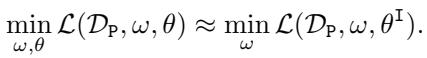
2. The Utility: We must not break the model’s ability to be fine-tuned on useful, safe tasks (\(\mathcal{D}_P\)). The condition number for the primary task should stay low.

3. The Performance: The model should still perform well on the original pre-training task.
The Linear Case
To make this theoretically tractable, the authors analyze linear models. They assume the feature extractor is a linear transformation \(\theta\). If the bad actor uses a Least Squares (\(\ell_2\)) loss, the optimization looks like this:
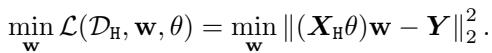
In this specific setting, the Hessian matrix of the loss function, which dictates the curvature of the loss landscape, has a closed form:

Here, \(\mathbf{K}_H\) is the covariance matrix of the harmful data. The authors derive a proposition showing that the singular values of this Hessian (\(\sigma_i\)) depend on the alignment between the singular vectors of the feature extractor \(\theta\) and the data covariance.
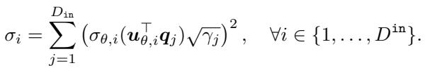
This equation confirms that by manipulating \(\theta\), we can control the singular values—and consequently the condition number—of the Hessian.
The Algorithm: Controlling the Condition Number
So, we have a plan: modify \(\theta\) during pre-training so that the Hessian for the harmful task is ill-conditioned (high \(\kappa\)) and the Hessian for the useful task is well-conditioned (low \(\kappa\)).
To do this via gradient descent, we need differentiable regularization terms that we can add to our loss function. The authors propose an objective function with three parts:

Let’s break down the two regularizers, \(\mathcal{R}_{ill}\) and \(\mathcal{R}_{well}\).
1. The “Well” Regularizer (\(\mathcal{R}_{well}\))
This term is adapted from prior work. It encourages the matrix to have a small condition number (making optimization easy). It essentially tries to keep the matrix close to a scaled identity matrix.

When we minimize this term, we are pushing the condition number down, ensuring the model remains useful for legitimate tasks.
2. The “Ill” Regularizer (\(\mathcal{R}_{ill}\))
This is the novel contribution of the paper. We need a way to maximize the condition number. However, the condition number itself is hard to optimize directly because it is non-convex and discontinuous.
The authors introduce \(\mathcal{R}_{ill}\), a differentiable proxy that upper-bounds the inverse of the log condition number.
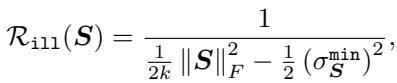
Let’s interpret this fraction. The denominator contains \(\|\mathbf{S}\|_F^2\) (the sum of squared singular values) minus a term involving the minimum singular value. By minimizing this whole term, we effectively drive the denominator toward zero, which happens when the condition number explodes toward infinity.
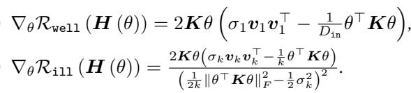
The authors prove that this regularizer is differentiable (under mild assumptions) and provide its gradient:
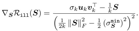
Crucially, they prove that taking gradient steps to minimize \(\mathcal{R}_{ill}\) is guaranteed to increase the condition number monotonically.
The Update Rule
With these regularizers defined, the immunization process becomes a modified training loop. We train the model on the primary task while simultaneously pushing the gradients to satisfy our condition number constraints.
The update rule for the feature extractor \(\theta\) looks like this:
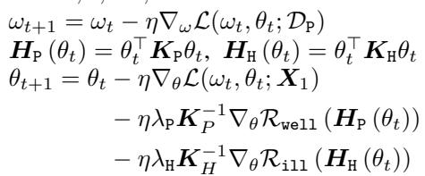
Notice the three components updating \(\theta_{t+1}\):
- The standard gradient from the task loss (\(\nabla_\theta \mathcal{L}\)).
- A term minimizing \(\mathcal{R}_{well}\) on the primary data (keeping it useful).
- A term minimizing \(\mathcal{R}_{ill}\) on the harmful data (making it resistant).
The authors also derive the specific gradients for these regularizers with respect to the feature extractor \(\theta\):
Experiments and Results
Does this mathematical theory hold up in practice? The researchers tested the algorithm on both linear models and deep neural networks.
To measure success, they introduced the Relative Immunization Ratio (RIR).
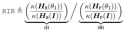
- Numerator (i): How much harder did we make the harmful task? (We want this high).
- Denominator (ii): How much harder did we make the useful task? (We want this low, ideally 1).
- Goal: An RIR \(\gg 1\).
Linear Models: House Prices and MNIST
First, they tested on a linear regression task (House Prices) and a classification task (MNIST).
House Prices: The table below compares their method (“Ours”) against baselines like “IMMA” (a previous bi-level optimization method) and “Opt \(\kappa\)” (direct optimization of condition number).
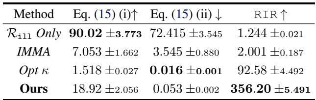
- Look at the RIR column: The proposed method achieves a massive RIR of 356.20.
- Look at (ii): The condition number ratio for the useful task is 0.053, meaning the useful task actually got easier to optimize (a happy side effect), while the harmful task became 18x harder (column i).
Convergence Speed: The chart below visualizes the “learning curve” (norm ratio) over time.
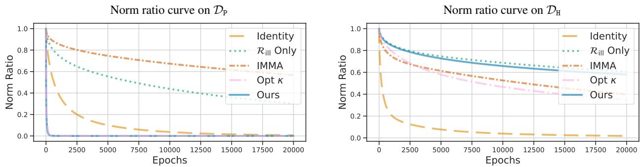
- Left (Primary Task): The blue line (Ours) drops the fastest. The model learns the useful task quickly.
- Right (Harmful Task): The blue line stays high. The model refuses to learn the harmful task effectively.
MNIST Heatmap: They also ran this on all pairs of digits in MNIST (e.g., make “1 vs 7” harmful, “3 vs 8” useful).
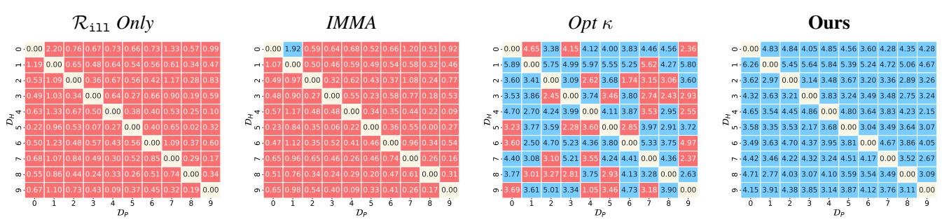
The grid on the far right (“Ours”) is almost entirely blue, indicating successful immunization across almost all digit combinations. The baselines (left grids) show a lot of red (failure).
Deep Networks: ImageNet
Finally, the authors applied this to deep non-linear models (ResNet18 and ViT) pre-trained on ImageNet. They treated ImageNet as the “safe” task and datasets like Stanford Cars or Country211 as the “harmful” tasks.
Since deep nets are non-linear, the Hessian isn’t exactly \(\theta^\top K \theta\), but we can approximate the effect by looking at the condition number of the feature representations.
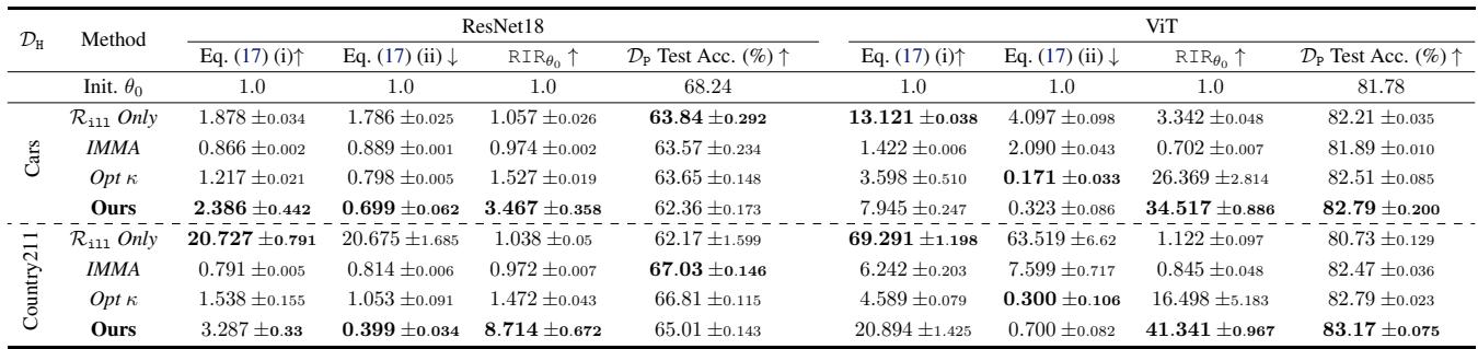
The results in Table 3 show that “Ours” consistently achieves the highest RIR. For example, with ViT on Stanford Cars, they achieve an RIR of 34.5, while maintaining (and even slightly improving) the test accuracy on ImageNet (82.79%).
The plot below shows the test accuracy on the harmful task during fine-tuning.
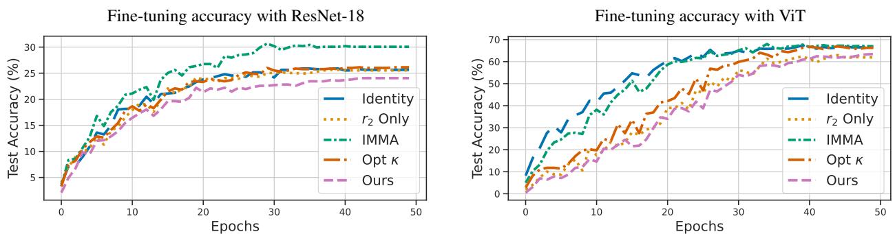
- Magenta Line (Ours): Notice how it lags behind the other lines. Even after many epochs of fine-tuning, the model immunized with this method yields the lowest accuracy on the harmful task. The immunization creates a “resistance” to learning the unwanted concept.
Conclusion and Implications
This paper bridges the gap between the empirical practice of model safety and the theoretical foundations of optimization. By viewing model immunization through the lens of the Condition Number, the authors provided:
- A precise definition of what it means for a model to be immunized.
- A novel regularizer (\(\mathcal{R}_{ill}\)) that provably maximizes the condition number.
- An algorithm that effectively protects both linear and deep models.
This “vaccine” for AI models suggests a future where open-source models can be released with a layer of mathematical protection, preventing bad actors from easily repurposing them for harm while keeping the scientific and commercial benefits of open access alive. While no defense is perfect, making the optimization landscape a “treacherous valley” for attackers is a powerful deterrent.