](https://deep-paper.org/en/paper/2505.24067/images/cover.png)
The intersection of classical algorithms and deep learning is one of the most fascinating frontiers in computer science. On one hand, we have classical algorithms—rigorous, interpretable, and guaranteed to work, but often rigid and unable to digest raw, messy real-world data. On the other hand, we have neural networks—flexible, adaptable, and capable of handling complex inputs, but often opaque and prone to hallucinating incorrect answers.
Neural Algorithmic Reasoning (NAR) attempts to fuse these two worlds. The goal is to train neural networks to “reason” like algorithms. By teaching a network to mimic the steps of a classical algorithm (like Breadth-First Search or Bellman-Ford), we hope to create systems that generalize better than standard deep learning models.
However, there has been a significant ceiling in this field. Most success stories in NAR have focused on “easy” problems—specifically, polynomial-time problems like sorting or finding shortest paths. But the real world is filled with hard problems—NP-hard problems—where finding an exact solution efficiently is impossible for large datasets.
In this post, we are doing a deep dive into a paper that tackles this ceiling head-on: “Primal-Dual Neural Algorithmic Reasoning.” This research introduces a framework called PDNAR, which aligns Graph Neural Networks (GNNs) with the powerful primal-dual method from combinatorial optimization.
What makes this approach unique? It doesn’t just mimic an algorithm; it learns to outperform the very approximation algorithm it was trained on, and it scales to massive graphs that it has never seen before.
The Challenge: Why NP-Hard is Hard for AI
To understand the contribution of this paper, we need to understand the gap in current research.
Previous NAR models effectively learned to execute algorithms like Prim’s algorithm for Minimum Spanning Trees. These are exact algorithms. If the model learns perfect execution, it gets the optimal answer.
But for NP-hard problems—like Vertex Cover or Set Cover—we don’t have efficient exact algorithms. We rely on approximation algorithms, which guarantee a solution within a certain factor of the optimum (e.g., “no worse than 2x the best possible cost”).
If we simply train a neural network to mimic an approximation algorithm, the best we can hope for is a model that is as good as that approximation. That’s not particularly useful. The researchers behind PDNAR asked a different question: Can we use the structure of approximation algorithms to build a neural network, but train it to find even better solutions?
Background: The Primal-Dual Paradigm
The core engine of this framework is the Primal-Dual method. This is a standard technique in designing approximation algorithms.
Every linear programming (LP) problem has a “dual” problem. If the “primal” problem is to minimize cost, the “dual” problem is to maximize profit (loosely speaking). The “Weak Duality Principle” states that any feasible solution to the dual problem provides a lower bound for the primal problem.
By iteratively updating variables in both the primal and dual problems, we can squeeze the gap between them, eventually arriving at a solution.
The Problems
The paper focuses on three classic NP-hard problems. Let’s look at their mathematical formulations to see the primal-dual structure.
1. Minimum Vertex Cover (MVC)
Imagine a graph. You want to select the smallest set of vertices such that every edge is connected to at least one selected vertex.
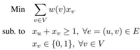
The dual of this problem involves “edge packing”—assigning weights to edges such that no vertex is “overloaded.”
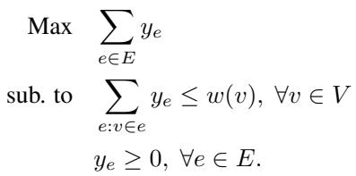
2. Minimum Set Cover (MSC) and Hitting Set Set cover is a generalization where you try to cover elements using a family of sets. The Hitting Set problem is mathematically equivalent but often easier to formulate generally. The goal is to pick the minimum weight of elements to “hit” every set.
In these formulations:
- Primal variables (\(x\)): Usually binary decisions (e.g., “Do I include this vertex?”).
- Dual variables (\(y\)): Constraints or costs associated with the connections.
An approximation algorithm typically works by gradually increasing the dual variables. When a constraint becomes “tight” (the dual pressure equals the weight of the item), the algorithm selects that item for the solution.
The PDNAR Framework
The researchers propose PDNAR (Primal-Dual Neural Algorithmic Reasoning). The genius of this approach lies in how it converts the mathematical relationship between primal and dual variables into a neural architecture.
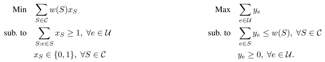
1. The Bipartite Representation
Instead of treating the input graph as a standard graph, PDNAR views the problem as a bipartite graph.
- Left Nodes (Primal): Represent the elements we might choose (e.g., vertices in Vertex Cover).
- Right Nodes (Dual): Represent the constraints we need to satisfy (e.g., edges that need covering).
An edge exists between a primal node and a dual node if that element is involved in that constraint.
2. The Architecture
The model follows the standard NAR “Encoder-Processor-Decoder” blueprint, but the Processor is specially designed to mimic the primal-dual updates.
Let’s break down the flow shown in the diagram above:
Step A: Encoding The model takes the current state of the solution. This includes the “residual weight” (\(r_e\)) of an element (how much “cost” is left before we are forced to pick it) and its degree (\(d_e\)). These are passed through Multi-Layer Perceptrons (MLPs) to create latent vectors.
 Note: In the implementation, logarithmic transformations are often used to handle varying scales.
Step B: The Processor (Algorithmic Alignment) This is the heart of the model. Standard GNNs just sum up neighbor features. PDNAR aligns its message passing with the specific mathematical operations of the primal-dual algorithm.
First, the dual nodes (constraints) gather information from the primal nodes. In the classical algorithm, this step involves finding a minimum ratio. Therefore, the GNN uses a min-aggregation function:
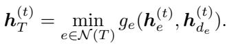
Next, the primal nodes update their status based on the feedback from the dual nodes. In the algorithm, this corresponds to reducing the residual weight of an element. The GNN mimics this using a summation:
Step C: The “Uniform Increase” Rule Some advanced approximation algorithms require a global update—increasing all dual variables simultaneously until something breaks. To support this, PDNAR introduces a virtual node (\(z\)) (seen in the architecture diagram).
- All dual nodes send messages to the virtual node (global aggregation).
- The virtual node sends a global signal back to the primal nodes.
This allows the network to learn complex, global reasoning steps that local message passing implies miss.
Step D: Decoding Finally, decoders translate the latent vectors back into predictions:
- \(\hat{x}_e\): Probability of picking this element (the solution).
- \(\hat{r}_e\): Predicted residual weight.
- \(\hat{\delta}_T\): Predicted dual variable update.

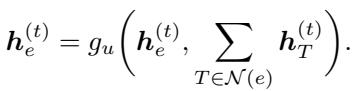
3. Theoretical Alignment
One of the paper’s strong contributions is a theoretical proof. The authors prove that there exists a set of weights for this neural network such that it exactly replicates the execution of the classical primal-dual algorithm.
By proving this algorithmic alignment, they ensure the model has the capacity to be at least as good as the approximation algorithm.
The equation above is part of the proof showing that specific weight configurations in the GNN result in the exact mathematical operation (\(r_e / d_e\)) found in the classical algorithm.
The Secret Sauce: Optimal Supervision
If the model only learned to mimic the approximation algorithm, it would just be a slower version of a standard script.
The authors introduce a hybrid training strategy:
- Algorithmic Trajectory: They train the model to predict the step-by-step changes of the approximation algorithm (mimicking the teacher).
- Optimal Supervision: For small graphs (e.g., 16 nodes), they run an exact solver (like Gurobi) to get the perfect solution. They add a loss term requiring the model’s final output to match this perfect solution.
Why does this matter? Approximation algorithms are “greedy”—they make locally optimal choices that might be suboptimal globally. By adding the Optimal Supervision signal, the neural network learns to leverage its parameters to “correct” the greedy mistakes of the algorithm. It learns the structure of the algorithm but the decision-making of the optimal solver.
Because it learns the structure, it generalizes to huge graphs. Because it learns the optimal decisions, it outperforms the original algorithm.
Experimental Results
The authors tested PDNAR on Vertex Cover (MVC), Set Cover (MSC), and Hitting Set (MHS).
1. Beating the Teacher
They trained the model on small graphs (16 nodes) and tested it on much larger graphs (up to 1024 nodes). The metric below is the Model-to-Algorithm Ratio.
- Ratio = 1.0: The model performs exactly as well as the approximation algorithm.
- Ratio < 1.0: The model found a better solution than the algorithm it mimicked.

Look at the PDNAR rows. The ratios are consistently below 1.0 (e.g., 0.915 for Set Cover). This confirms the hypothesis: the model learned to improve upon the approximation logic. Note that standard GNNs (GIN, GAT) often fail to generalize to larger graphs (ratios > 1.0), while PDNAR remains stable as graph size grows exponentially.
2. Generalization to New Graph Types
A common failure mode for AI is “Out-Of-Distribution” (OOD) failure. A model trained on random graphs might fail on “star” graphs or “planar” graphs.
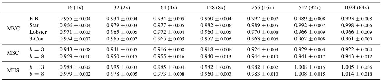
The results above show that PDNAR generalizes exceptionally well. Even when trained on Barabási-Albert graphs, it handles Star graphs and Lobster graphs effectively (ratios still < 1.0 or very close). This suggests the model has learned the underlying algorithm, not just dataset statistics.
3. Real-World Application: Airport Traffic
The authors applied PDNAR to real-world airport datasets to predict airport activity levels (a node classification task). They used PDNAR to generate embeddings based on the vertex cover structure and concatenated them with standard GNN embeddings.
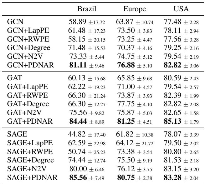
Adding PDNAR features (GAT+PDNAR) consistently improved accuracy over the baselines. This proves that “algorithmic features” (knowing how important a node is in a vertex cover sense) are valuable for general learning tasks.
4. Practical Engineering: Warm-Starting Solvers
This is perhaps the most immediate practical application. Commercial solvers like Gurobi are used in logistics and finance to solve integer programs. They are fast, but they get slower as problems get massive.
You can speed up Gurobi by giving it a “warm start”—a good initial guess. The authors used PDNAR to generate a guess and fed it into Gurobi.
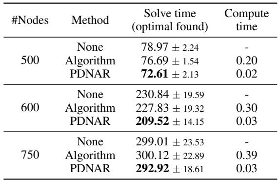
As shown in the table:
- Solve Time: Using PDNAR to warm-start Gurobi (bottom row of each section) resulted in the fastest solve times.
- Compute Time: It takes the neural network fractions of a second (0.03s) to generate the guess, whereas running the classical approximation algorithm took much longer (0.39s for 750 nodes).
The neural network is essentially acting as a lightning-fast heuristic generator that makes exact solvers more efficient.
Conclusion
The “Primal-Dual Neural Algorithmic Reasoning” paper presents a significant step forward in our ability to use neural networks for hard combinatorial problems.
By strictly aligning the neural architecture with the bipartite primal-dual structure, the model gains the robustness of classical algorithms. By training with optimal supervision on small instances, it gains the intuition of exact solvers.
Key Takeaways:
- Structure Matters: You cannot just throw a standard Transformer or GNN at an NP-hard problem and expect it to reason. The architecture must mirror the problem’s mathematical structure.
- Small Data, Big Generalization: You can train on small, cheap-to-solve graphs and deploy on massive, expensive-to-solve graphs.
- Better than the Original: A neural network can learn to mimic an algorithm and then, via gradient descent and optimal labels, learn to fix the algorithm’s greedy mistakes.
This framework opens the door for hybrid systems where neural networks don’t replace classical solvers, but rather augment them—providing high-quality approximations instantly and accelerating the search for exact solutions.