](https://deep-paper.org/en/paper/2505.24688/images/cover.png)
Beyond Temperature: Guiding LLM Thoughts with Soft Reasoning and Bayesian Optimization
If you have ever tried to get a Large Language Model (LLM) to solve a complex math problem or a tricky logic puzzle, you likely know the frustration of “hallucinations” or lazy reasoning. You ask a question, and the model confidently gives you the wrong answer.
To fix this, we often rely on two main strategies. The first is Prompt Engineering—telling the model to “think step by step” (Chain-of-Thought). The second is Decoding Strategies—specifically, adjusting the “temperature.” If the model is stuck, we raise the temperature to increase randomness, hoping that in a batch of 10 or 20 generated answers, one will be correct.
But is cranking up the randomness really the best way to explore solutions? High temperature is a blunt instrument; it flattens the probability distribution, making the model just as likely to say something nonsensical as it is to find a creative solution.
A fascinating new paper titled Soft Reasoning: Navigating Solution Spaces in Large Language Models through Controlled Embedding Exploration proposes a smarter way. Instead of randomly shaking the model (temperature) or begging it to try harder (prompting), the researchers introduce a method to mathematically steer the model’s internal “thought process” using Bayesian Optimization.
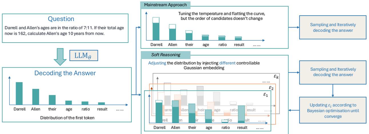
As shown in Figure 1, while mainstream approaches rely on random sampling, Soft Reasoning injects precise, controlled noise into the model’s embeddings and optimizes that noise to find the best possible answer. In this post, we will tear down this architecture to understand how we can control LLM reasoning without ever touching the model’s weights.
The Problem with Current Decoding
To understand why Soft Reasoning is necessary, we first need to look at how LLMs generate text. At every step, the model predicts a probability for every word in its vocabulary.
In Greedy Decoding, the model always picks the most probable word. This is stable but repetitive. It often gets stuck in “local optima”—if the first step of a math problem is slightly wrong, the whole solution fails.
To fix this, we usually use Temperature Scaling. The probability of selecting a token \(w^{(t)}\) at time step \(t\) is adjusted by a temperature parameter \(\tau\):
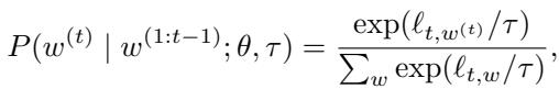
When \(\tau\) is high, the distribution flattens. Low-probability words become more likely. This creates diversity, but it is “blind” diversity. The model doesn’t know which low-probability words are clever pivots and which are just gibberish.
More advanced methods, like Tree of Thoughts (ToT) or Monte Carlo Tree Search (MCTS), try to explore different reasoning paths explicitly. However, these are computationally expensive and rely heavily on the text prompts themselves. If the prompt isn’t perfect, the search is a “wild-goose chase.”
The Core Concept: The Butterfly Effect of Embeddings
The authors of Soft Reasoning propose a shift in perspective. Instead of manipulating the output probabilities (like temperature does), why not manipulate the input representation of the solution?
The hypothesis is simple: The first token generated in an answer determines the trajectory of the entire reasoning path.
If we can nudge the “meaning” of that first token just slightly in the high-dimensional embedding space, we can steer the model toward a completely different, potentially correct, line of reasoning.
Step 1: Embedding Perturbation
Normally, an LLM selects the first token \(w^{(1)}\) based on the prompt \(q\) using greedy decoding:
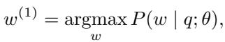
Let \(z\) be the continuous vector embedding of this chosen token. Soft Reasoning adds a small amount of Gaussian noise to this embedding. Instead of using the exact embedding \(z\), the model uses a perturbed version \(x_i\):
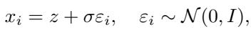
Here, \(\varepsilon_i\) is random noise, and \(\sigma\) controls how strong the nudge is.
Crucially, only the first token’s embedding is perturbed. Once this specific, slightly shifted “concept” is fed into the model, the rest of the sequence is generated using Greedy Search:
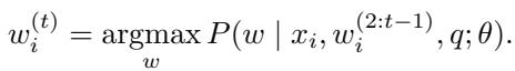
This is a vital distinction. In standard temperature sampling, every step is random. In Soft Reasoning, the “seed” (the perturbed embedding) is random, but the resulting growth (the text generation) is deterministic. This means every specific noise vector \(x_i\) maps to a unique, repeatable reasoning path.
Step 2: The Soft Reasoning Framework
Now that we can generate diverse answers by tweaking the embedding, we have a search problem. The embedding space is infinite. Where do we look for the best answer?
We treat the LLM as a “black box” function where the input is the perturbation vector and the output is the quality of the answer. We can then use Bayesian Optimization (BO) to find the optimal perturbation.
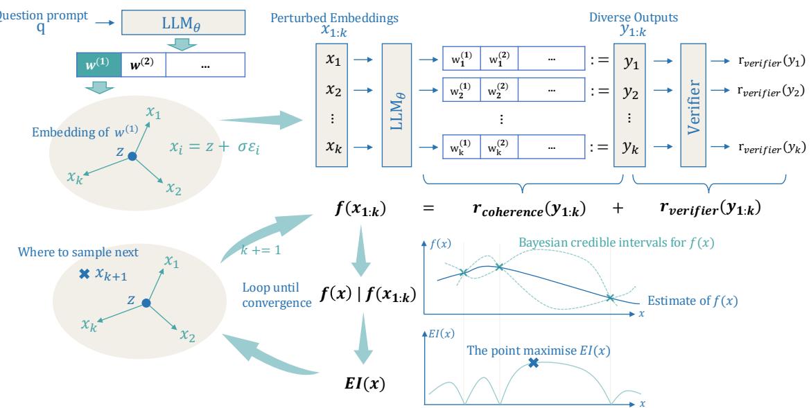
As illustrated in Figure 2, the process works in a loop:
- Perturb: Generate a set of candidate embeddings \(x_{1:k}\).
- Generate: The LLM produces answers \(y_{1:k}\) based on those embeddings.
- Evaluate: A reward function scores the answers.
- Optimize: A Bayesian model looks at the scores and decides where to search next.
Step 3: Defining the Reward
To optimize the reasoning, we need to mathematically define what a “good” answer looks like. The authors define an objective function \(f(x)\) composed of two parts:
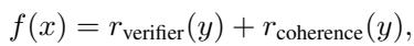
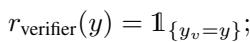
1. The Verifier (\(r_{\text{verifier}}\)): This checks if the answer is correct. In this framework, the authors simply use the LLM itself (or another model) to verify the result.
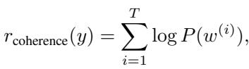
2. Coherence (\(r_{\text{coherence}}\)): If we perturb an embedding too much, the model might generate nonsense. The coherence score ensures the text is fluent by checking the probability of the tokens generated.
The combination ensures that the optimization seeks answers that are both factually correct (according to the verifier) and linguistically sound.
Step 4: Bayesian Optimization and Expected Improvement
This is where the method shines. Randomly trying perturbations is inefficient. Bayesian Optimization builds a probabilistic model (a surrogate model) of how the embedding space maps to the reward.
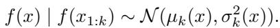
It assumes the function \(f(x)\) follows a Gaussian Process. This allows the system to predict the mean reward \(\mu\) and the uncertainty \(\sigma\) for any point in the embedding space.

After observing a few samples, the model updates its belief:
To decide where to sample next, the algorithm uses an acquisition function called Expected Improvement (EI).
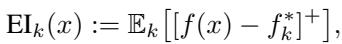
In simple terms, EI balances Exploration (looking in areas where uncertainty \(\sigma\) is high) and Exploitation (looking in areas where the predicted reward \(\mu\) is high). It asks: “How much better do we expect this new point to be compared to the best result we’ve found so far?”
The closed-form solution for this is efficient to compute:
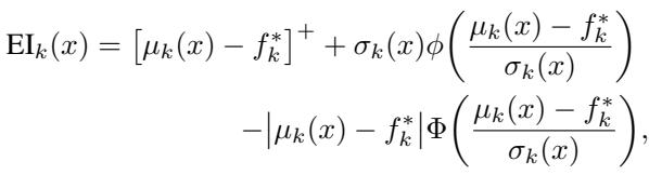
By maximizing this value, Soft Reasoning intelligently navigates the embedding space, converging on the “critical neurons” and representations that yield the correct answer.
Experimental Results
The researchers tested Soft Reasoning against several strong baselines, including Self-Consistency (SC) and Planning-based methods like RAP, on difficult benchmarks like GSM8K (math) and StrategyQA (commonsense reasoning).
Accuracy
The results are impressive. As shown in Table 1 below, Soft Reasoning consistently outperforms standard decoding and Self-Consistency, specifically in zero-shot settings where the model has no examples to rely on.
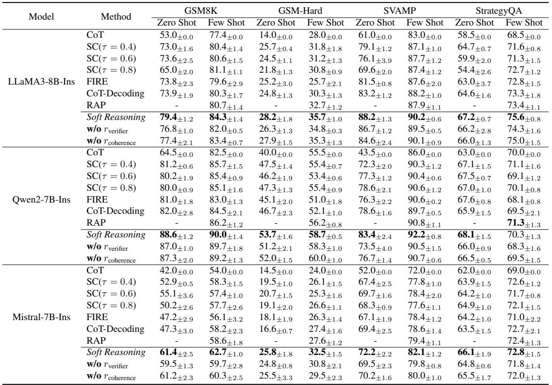
For example, on the GSM8K dataset using LLaMA-3-8B, Soft Reasoning achieved 79.4% accuracy in zero-shot, compared to 73.0% for Self-Consistency (\(\tau=0.4\)). It essentially squeezes more reasoning power out of the same model parameters.
Efficiency
One of the biggest criticisms of “Tree of Thoughts” or other planning algorithms is that they are slow and token-hungry. They generate thousands of intermediate thoughts.
Soft Reasoning is far lighter. Because it operates on the embedding of a single token and uses an efficient mathematical optimizer, it drastically reduces computational overhead.
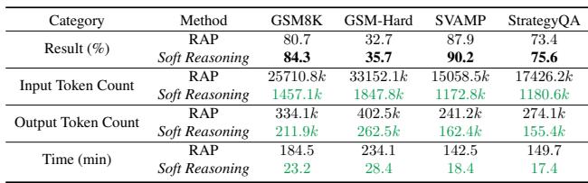
Table 3 highlights this efficiency gap. Compared to RAP (a tree-search method), Soft Reasoning uses roughly 6% of the input tokens and runs nearly 8 times faster (23 minutes vs. 184 minutes for the test set), all while achieving higher accuracy (84.3% vs 80.7%).
Convergence
Does the Bayesian Optimization actually learn anything? Or is it just getting lucky?
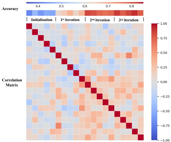
Figure 5 shows the correlation matrix of the sampled points evolving over iterations. As the process continues, the matrix becomes more structured, indicating that the algorithm is identifying a specific region in the embedding space that correlates with high rewards. It isn’t just guessing; it’s narrowing down the search.
Why Does It Work? The Neural Perspective
The most fascinating part of the paper is the analysis of why perturbing embeddings works better than temperature sampling. The authors looked at the activation rates of neurons inside the LLM’s MLP (feed-forward) layers.
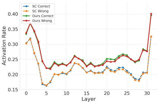
Figure 3 compares the neuron activation rates of Soft Reasoning (Ours) versus Self-Consistency (SC).
- SC (Blue/Orange): The activation rates drop significantly in the middle layers.
- Soft Reasoning (Green/Red): Maintains a more stable, higher activation rate across layers.
This suggests that embedding perturbation triggers a broader set of neural pathways. The authors even identified “critical neurons”—specific neurons that are highly correlated with correct answers.
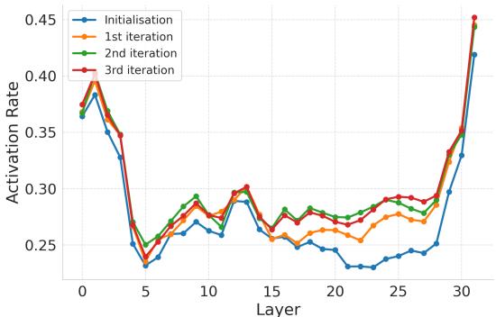
In Figure 4, we see that as the Bayesian Optimization iterates (going from Initialization to the 3rd iteration), the activation rate of these critical neurons increases. The optimization process effectively “finds” the part of the model’s brain needed to solve the problem and forces it to activate.
Conclusion and Implications
Soft Reasoning represents a sophisticated step forward in how we interact with Large Language Models. Rather than treating the model as a rigid box that we must “prompt” correctly, or a chaotic box that we must “sample” randomly, this approach treats the model’s latent space as a landscape to be explored.
By combining the continuous nature of embeddings with the rigorous search capability of Bayesian Optimization, the authors offer a method that is:
- Model-Agnostic: It works without retraining the LLM.
- Efficient: It requires far fewer tokens than tree-search methods.
- Effective: It activates critical reasoning pathways that standard decoding misses.
For students and researchers, this highlights an exciting direction: Latent Space Optimization. As models get larger and harder to retrain, techniques that optimize the inputs and internal states at inference time—like Soft Reasoning—will likely become the standard for tackling complex reasoning tasks.