Taming the Combinatorial Explosion with Probabilistic Experimental Design

Imagine you are a biologist trying to understand how a cell works. You suspect that knocking out specific genes will change the cell’s state, perhaps turning a cancer cell into a benign one. You have 20 different genes you can target.

If you test one gene at a time, you have 20 experiments. That’s manageable. But biology is rarely linear; genes interact. One gene might do nothing on its own, but if paired with another, it could be lethal to the cell. To fully understand the system, you need to test combinations.

Here lies the problem: The Combinatorial Explosion.

With 20 genes, the number of possible combinations (a “full factorial” design) is \(2^{20}\), which is over a million experiments. In a wet lab, that is impossible. You need a way to run a manageable number of experiments—say, 1,000—while still learning as much as possible about how these genes interact.

This is the problem addressed in the research paper “Probabilistic Factorial Experimental Design for Combinatorial Interventions” by Divya Shyamal, Jiaqi Zhang, and Caroline Uhler.

In this post, we will dive deep into their proposed framework: Probabilistic Factorial Design. We will explore how assigning probabilities (dosages) to treatments, rather than hand-picking combinations, offers a scalable, theoretically grounded way to learn complex interactions without running a million experiments.

The Design Dilemma: Full vs. Fractional

Before looking at the new solution, let’s understand the status quo.

1. Full Factorial Design: You test every possible combination.

• Pros: You get perfect data on all interactions.
• Cons: Mathematically impossible to scale. The number of experiments grows exponentially with the number of treatments (\(p\)).

2. Fractional Factorial Design: You select a specific subset of combinations to test.

• Pros: Uses fewer samples.
• Cons: It is rigid. You have to carefully select which combinations to run to avoid “aliasing” (confounding different interactions). If you design it wrong, you might think Gene A and Gene B are interacting when it’s actually Gene C acting alone. Designing these experiments requires heavy prior assumptions (e.g., “I assume there are no 3-way interactions”).

The authors of this paper propose a third way, inspired by how high-throughput biological screens (like Perturb-seq) are actually performed. Instead of explicitly choosing “Row 1 gets Gene A and B,” they propose a probabilistic approach.

The Probabilistic Framework

The core idea is simple but powerful. Instead of assigning a fixed combination of treatments to a unit (e.g., a cell), the experimenter chooses a dosage vector \(\mathbf{d} = (d_1, \dots, d_p)\).

Each \(d_i\) represents the probability that treatment \(i\) is applied. For every experimental unit \(m\), the treatment assignments are drawn randomly based on these probabilities.

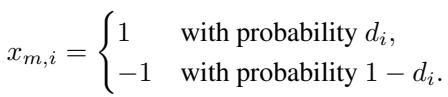
Mathematically, let \(x_{m,i}\) be the intervention status of treatment \(i\) on unit \(m\). It takes a value of 1 (treatment applied) or -1 (control/not applied).

Here is why this is clever:

• If you set \(\mathbf{d} \in \{0, 1\}^p\), you recover the traditional deterministic design.
• If you set \(\mathbf{d} \in (0, 1)^p\), you create a stochastic design where you explore the combinatorial space randomly.

By adjusting the continuous parameter \(\mathbf{d}\), the experimenter can control the “center of gravity” of the experiments without having to explicitly enumerate every combination.

Modeling Combinatorial Outcomes

To optimize the design, we need a mathematical model of the world. How do inputs (treatments) map to outputs (outcomes)?

The authors define the outcome \(y_m\) for unit \(m\) as a function of the treatment vector \(\mathbf{x}_m\) plus some noise:

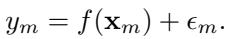
The function \(f\) could be anything. However, to analyze interactions, the authors use the Fourier expansion for Boolean functions. While “Fourier” usually reminds us of sine waves, in the context of binary inputs (\(\{-1, 1\}\)), the Fourier basis functions are simply products of the inputs.

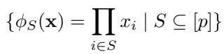
For any subset of treatments \(S \subseteq [p]\), the basis function is:

This looks abstract, so let’s make it concrete.

• If \(S = \{1\}\), then \(\phi_S(\mathbf{x}) = x_1\). This measures the main effect of Treatment 1.
• If \(S = \{1, 2\}\), then \(\phi_S(\mathbf{x}) = x_1 x_2\). This measures the pairwise interaction between Treatment 1 and 2.

Any function \(f\) can be written as a weighted sum of these interactions:

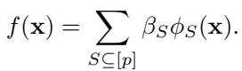
Here, \(\beta_S\) represents the strength of the interaction for the set \(S\). If \(\beta_{\{1,2\}}\) is large, it means Genes 1 and 2 have a strong synergy (or antagonism).

Connection to Polynomial Models

This Fourier approach is equivalent to a standard polynomial response surface model often used in statistics. If you are used to seeing interaction terms like \(\alpha_{ij} \mathbb{1}_{x_i=x_j=1}\), these can be directly mapped to the Fourier coefficients \(\beta_S\).

The relationship between the standard coefficients (\(\alpha\)) and the Fourier coefficients (\(\beta\)) is linear:

Bounded Interactions

In the real world, we rarely see 10 distinct genes all interacting simultaneously in a unique way that cannot be explained by lower-order effects. The authors assume bounded-order interactions. We assume that interactions only exist up to size \(k\) (e.g., \(k=2\) or \(k=3\)).

This assumption is crucial because it reduces the number of parameters we need to estimate from \(2^p\) down to something polynomial in \(p\), making the problem solvable.

The Passive Setting: The “Set It and Forget It” Strategy

The first major contribution of the paper addresses the passive setting. You have a budget of \(n\) samples. You need to choose a dosage vector \(\mathbf{d}\) once, at the beginning. What dosages should you pick to estimate the model coefficients \(\boldsymbol{\beta}\) as accurately as possible?

To answer this, we look at the estimator. We want to recover \(\boldsymbol{\beta}\) from our data observations. The design matrix \(\mathcal{X}\) contains the Fourier features for every sample:

Since our design is random, the matrix \(\mathcal{X}\) might be ill-conditioned (some columns might be correlated by chance). To handle this, the authors use a Truncated Ordinary Least Squares (OLS) estimator. Essentially, it performs standard linear regression but “gives up” (returns zero) if the matrix is too unstable (i.e., eigenvalues are too small) to avoid massive variance.

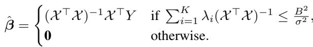
The Metric: Mean Squared Error

We want to minimize the expected Mean Squared Error (MSE) between our estimated coefficients \(\hat{\boldsymbol{\beta}}\) and the true \(\boldsymbol{\beta}\). The theoretical bounds for this error depend heavily on the eigenvalues (\(\lambda_i\)) of the matrix \(\mathcal{X}^\top \mathcal{X}\).

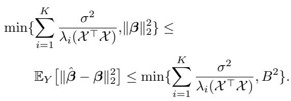
The term \(\sum \frac{1}{\lambda_i}\) is the key. In linear regression, the variance of the estimator is proportional to the trace of the inverse covariance matrix. To minimize error, we want large eigenvalues.

The Optimal Strategy

Here is the striking result of the paper. Under the probabilistic design framework, for any interaction order \(k\):

The optimal dosage is \(\mathbf{d} = (1/2, 1/2, \dots, 1/2)\).

This means essentially flipping a fair coin for every treatment on every unit.

Why is \(1/2\) optimal? It comes down to the population covariance matrix, denoted as \(\Sigma(\mathbf{d})\). The entries of this matrix are determined by the dosages:

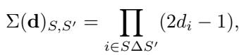
The eigenvalues of this matrix dictate the error. The sum of the eigenvalues is constant regardless of \(\mathbf{d}\). By a property of the harmonic mean (Cauchy-Schwarz inequality), the sum of inverse eigenvalues is minimized when all eigenvalues are equal.

When \(\mathbf{d} = 1/2\), the term \((2d_i - 1)\) becomes 0. This collapses the covariance matrix \(\Sigma(\mathbf{d})\) into the Identity Matrix. The identity matrix has all eigenvalues equal to 1. This is the perfect condition for regression—it means all your features (interactions) are perfectly uncorrelated with each other.

The authors prove that the dosage \(1/2\) is optimal up to a very small factor:

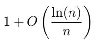
Specifically, the error rate decays with the sample size \(n\) as:

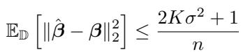
This implies that to estimate a \(k\)-way interaction model, you need roughly \(O(k p^{3k} \ln p)\) samples. This is polynomial, not exponential, which is a massive win for scalability.

The Active Setting: Learning on the Fly

In many scientific scenarios, you don’t run all experiments at once. You run a batch, analyze the data, and then design the next batch. This is Active Learning.

Suppose we have conducted \(T-1\) rounds of experiments. We have collected data matrices \(\mathcal{X}_1, \dots, \mathcal{X}_{T-1}\). We want to choose the dosage \(\mathbf{d}_T\) for the next round to minimize our total error.

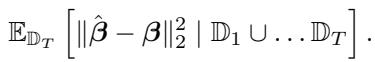
Since we already have data, our current “information” is represented by the sum of the gram matrices \(\mathcal{X}^\top \mathcal{X}\) from previous rounds. We might have gathered biased data by chance, or perhaps we were forced to use suboptimal dosages in round 1. Round \(T\) is our chance to “correct” the covariance structure.

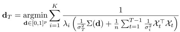
The authors derive a near-optimal acquisition function. We select the dosage \(\mathbf{d}_T\) that minimizes the inverse eigenvalues of the combined covariance (past data + expected new data):

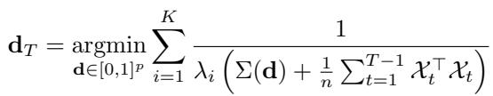
This formula cannot be solved in closed form like the passive setting, but it is a smooth function of \(\mathbf{d}\). This means we can use numerical optimization (like gradient descent or SLSQP) to find the best dosages for the next round.

This is a powerful tool. It allows the experiment to “fill in the holes” of the information space dynamically.

Extensions: Real-World Constraints

The paper extends this framework to several practical scenarios.

1. Limited Supply

What if reagents are expensive, or applying too many treatments simultaneously kills the cell? We might impose a constraint that the sum of dosages cannot exceed a limit \(L\):

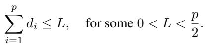
For a simple additive model (\(k=1\)), the authors prove that the optimal strategy is to spread the budget evenly, setting \(d_i = L/p\) for all treatments. For higher-order interactions, the numerical optimizer (from the active setting) can respect this constraint and find the best solution.

2. Heteroskedastic Noise

What if different rounds of experiments have different noise levels (\(\sigma_t^2\))? Perhaps the lab equipment was recalibrated, or a different batch of cells was used. The optimization function naturally adapts to this by weighting the covariance matrices by their precision (\(1/\sigma^2\)):

3. Emulating a Target Distribution

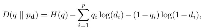
Sometimes, you don’t just want to minimize regression error. You might want your experimental population to mimic a specific distribution of combinations \(q\) found in nature.

The authors show that by minimizing the KL divergence between the target distribution \(q\) and the design distribution \(p_{\mathbf{d}}\), the optimal dosage is simply the marginal probability of the target distribution.

Experimental Validation

The theory is sound, but does it work in practice? The authors performed simulations to validate their claims.

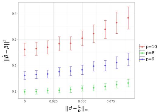
Simulation 1: Is 1/2 really optimal?

In this experiment, they fixed a “true” model and tried to estimate it using different dosage vectors. They varied the distance of the dosage vectors from the theoretical optimum of \(0.5\).

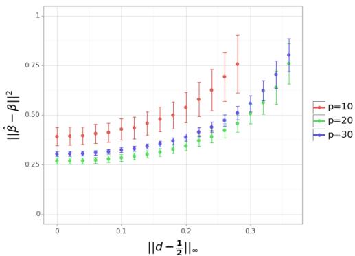
Interpretation: Look at Figure 1. The x-axis represents the distance from the dosage \(0.5\). The y-axis is the estimation error. The curve clearly goes up as you move away from 0.5. This empirically confirms the theorem: the “fair coin flip” (0.5) minimizes error.

Simulation 2: Uniform Dosages

They also tested setting all dosages to the same value \(d\), varying \(d\) from 0.4 to 0.6.

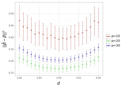
Interpretation: Figure 2 shows a clear “U” shape centered exactly at 0.5. Deviating even slightly (e.g., to 0.4 or 0.6) increases the error, reinforcing the sensitivity and optimality of the half-dosage strategy in the passive setting.

Simulation 3: Active vs. Random

Here, they compared the Active strategy (optimizing the dosage each round) against a Random strategy (picking random dosages) and a fixed Half strategy.

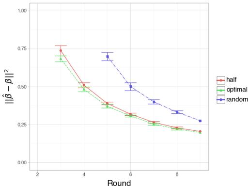
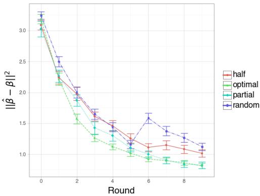
Interpretation:

• Figure 3 (Large \(N\)): With enough samples, the “Half” strategy (Red) and “Optimal” active strategy (Green) perform similarly well, both beating Random (Blue). This makes sense; if you have enough data, the passive optimal strategy is hard to beat.
• Figure 4 (Small \(N\), High Noise): This is the interesting case. When data is scarce, the Optimal strategy (Green) significantly outperforms the others in early rounds. It suggests that when experiments are expensive (small sample size), calculating the exact optimal dosage using the active learning framework provides a significant advantage.

Simulation 4: Constrained Optimization

Finally, they tested the limited supply scenario where the sum of dosages is constrained.

Interpretation: The error increases as the dosage deviates from the uniform distribution of the available budget (\(L/p\)). This confirms that even under constraints, spreading your resources evenly is generally the best starting policy for learning interactions.

Conclusion and Key Takeaways

The paper “Probabilistic Factorial Experimental Design for Combinatorial Interventions” provides a rigorous mathematical foundation for a problem that plagues many experimental sciences: how to study complex combinations without testing everything.

Key Takeaways:

1. Probabilistic Design: Moving from discrete selection of combinations to continuous “dosages” makes the design problem differentiable and scalable.
2. The Power of 1/2: In a passive (one-shot) experiment, setting every treatment probability to 50% is theoretically near-optimal for learning interactions of any order. It makes the features uncorrelated.
3. Active Correction: If doing experiments in rounds, you can numerically optimize dosages to correct for past imbalances or constraints, which is particularly valuable when sample sizes are small.
4. Flexibility: This framework naturally handles constraints (budget limits) and variations in experimental noise.

For students and researchers, this work bridges the gap between classical experimental design (which can be too rigid) and modern high-throughput capabilities. It suggests that sometimes, the best way to understand a complex deterministic system is to probe it with randomness.