Breaking the Tabular Barrier: How TABFLEX Scales Transformers to Millions of Rows

Introduction

If you have taken an introductory machine learning course, you likely know the golden rule of tabular data: Gradient Boosted Decision Trees (GBDTs) are king. While Deep Learning has revolutionized images (CNNs, ViTs) and text (LLMs), tabular data—the rows and columns that make up the vast majority of business and medical databases—has remained the stronghold of XGBoost, LightGBM, and CatBoost.

However, recent research has attempted to challenge this dominance using Transformers. The most notable attempt was TABPFN (Tabular Prior-Data Fitted Network), a model that acts like a “Large Language Model for tables.” Instead of training a model on your dataset, you simply feed your training data into the prompt (In-Context Learning), and it predicts the test labels immediately. It was revolutionary, but it had a massive flaw: Scalability. Because it relied on standard attention mechanisms, its computational cost exploded quadratically as the number of samples increased. It was brilliant for 1,000 rows, but useless for 100,000.

Enter TABFLEX.

In this post, we will dive into a new paper that proposes a solution to the tabular scaling problem. By replacing standard Softmax Attention with Linear Attention, TABFLEX reduces the computational complexity from quadratic to linear. The result? A model that can classify a million rows in under 5 seconds, outperforming XGBoost in efficiency while maintaining state-of-the-art accuracy.

The Problem: The Cost of Context

To understand why TABFLEX is necessary, we first need to understand the architecture it builds upon: TABPFN.

TABPFN treats tabular classification as an In-Context Learning (ICL) problem. Just as you might prompt GPT-4 with a few examples of English-to-French translation before asking it to translate a new sentence, TABPFN takes your entire training dataset (features and labels) and your test set (features only) and feeds them into a Transformer as a single sequence.

Figure 1: The architecture of TABPFN. The entire training set is fed into the model as a sequence. The model uses attention to learn the relationship between training examples and test examples in a single forward pass.

As shown in Figure 1, the model embeds the features (\(x\)) and labels (\(y\)) and processes them through a Transformer encoder. The key advantage here is that no gradient updates happen during inference. You don’t “train” the model on your data; the model “learns” the pattern instantly via the attention mechanism.

The Quadratic Wall

The Achilles’ heel of this approach is the standard Self-Attention mechanism (often called Softmax Attention). For a sequence of length \(N\), standard attention requires calculating an attention matrix of size \(N \times N\).

If you have 1,000 samples, the complexity is proportional to \(1,000^2\) (\(1,000,000\)). If you scale up to 10,000 samples, the complexity becomes \(10,000^2\) (\(100,000,000\)). This quadratic scaling (\(O(N^2)\)) makes it computationally impossible to feed large datasets into the prompt. TABPFN was effectively capped at a few thousand samples, rendering it unusable for “real-world” big data tasks.

The Search for a Scalable Architecture

The authors of TABFLEX set out to find an attention mechanism that scales linearly—\(O(N)\)—allowing them to process millions of samples. They investigated two primary candidates for scalable architectures: State-Space Models (SSMs/Mamba) and Linear Attention.

Investigation 1: State-Space Models (Mamba) vs. Transformers

State-Space Models (SSMs), particularly Mamba, have recently gained fame for matching Transformer performance on language tasks with linear scaling. It seems like a perfect fit, right?

The researchers found that the answer is no. The fundamental issue lies in Causality.

SSMs and Mamba are inherently causal (autoregressive). They process data sequentially, where token \(t\) can only see tokens \(0\) to \(t-1\). This makes sense for language (you read left-to-right) or audio (time moves forward). However, tabular data is permutation invariant. The order in which you feed rows into a model should not matter. Row 100 holds just as much relevant information for Row 1 as Row 2 does.

Figure 2: The impact of causal vs. non-causal masking. The non-causal model (blue) continues to improve as it sees more samples. The causal model (pink), which mimics Mamba’s constraints, plateaus and even degrades.

As Figure 2 illustrates, enforcing causality hurts tabular performance. A causal model effectively ignores “future” rows in the sequence, wasting valuable context. When the authors tested a Mamba-based architecture against the Transformer architecture, the results were clear:

Figure 3: Mamba vs. Transformer on tabular tasks. The Transformer (Non-causal) achieves significantly lower loss and higher AUC.

Investigation 2: Linear Attention

Since causal models failed, the authors turned to Linear Attention. To understand this, we need to look at the math.

Standard Softmax Attention calculates output \(\mathbf{a}_i\) using Query (\(Q\)), Key (\(K\)), and Value (\(V\)) vectors. It uses a softmax function to normalize the similarity scores:

\[ \text{Softmax Attention: } \mathbf{a}_{i} = \frac{\sum_{j=1}^{n} \exp\left(\mathbf{q}_{i}^{\top} \mathbf{k}_{j}\right) \cdot \mathbf{v}_{j}}{\sum_{j=1}^{n} \exp\left(\mathbf{q}_{i}^{\top} \mathbf{k}_{j}\right)} \]

The \(\exp(\mathbf{q}^\top \mathbf{k})\) term locks the query and key together inside a non-linear function, forcing us to compute the full \(N \times N\) matrix.

Linear Attention removes the softmax. Instead, it applies a feature mapping function \(\phi(\cdot)\) (like elu(x) + 1) individually to \(Q\) and \(K\). This allows us to use the associative property of matrix multiplication:

\[ \text{Linear Attention: } \mathbf{a}_{i} = \frac{\phi\left(\mathbf{q}_{i}\right)^{\top} \sum_{j=1}^{n} \phi\left(\mathbf{k}_{j}\right) \cdot \mathbf{v}_{j}}{\phi\left(\mathbf{q}_{i}\right)^{\top} \sum_{j=1}^{n} \phi\left(\mathbf{k}_{j}\right)} \]

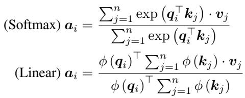
Why does this matter? In Linear Attention, we can compute \(\sum_{j=1}^{n} \phi(\mathbf{k}_{j}) \cdot \mathbf{v}_{j}\) first. This summation results in a matrix of size \(D \times D\) (where \(D\) is the embedding dimension, usually small), completely independent of the sequence length \(N\).

• Softmax Attention: \(O(N^2 D)\)
• Linear Attention: \(O(N D^2)\)

Since \(N\) (number of samples) is usually much larger than \(D\) (embedding size), Linear Attention is vastly more efficient for large datasets.

The researchers implemented this and found that Linear Attention maintained the accuracy of Softmax Attention while drastically cutting runtime.

Figure 4: Replacing Softmax with Linear Attention retains accuracy (y-axis) while significantly reducing runtime (x-axis).

TABFLEX: The Architecture

With the decision to use Non-Causal Linear Attention made, the authors developed TABFLEX.

Hardware Efficiency

Theoretical complexity (\(O(N)\)) doesn’t always translate to real-world speed if the GPU implementation is poor. The authors analyzed the High Bandwidth Memory (HBM) access patterns. They demonstrated that a straightforward PyTorch implementation of Linear Attention is actually highly efficient, matching the memory access complexity of highly optimized kernels like FlashAttention, without needing complex custom CUDA code.

Figure 5: Computational time (a) and Memory usage (b). Notice how standard FlashAttention (black dashed) still spikes in memory or time depending on settings, while Linear Attention (pink solid) scales linearly and efficiently across sequence lengths.

Conditional Model Selection

One model size does not fit all tabular problems. A dataset might have 50 rows and 20 features, or 1,000,000 rows and 1,000 features. TABFLEX utilizes a suite of three specialized models, routed based on the dataset’s shape:

1. TABFLEX-S100: Optimized for small datasets (\(<3k\) samples, \(<100\) features).
2. TABFLEX-L100: Optimized for long sequences (\(>3k\) samples, \(<100\) features).
3. TABFLEX-H1K: Optimized for high-dimensional data (\(1,000\) features).

This ensures that the model isn’t wasting compute on small data, nor is it under-powered for massive datasets.

Experimental Results

The results of TABFLEX are stunning, particularly when compared to its predecessor TABPFN and traditional Gradient Boosting methods.

1. Speed and Scalability

On standard validation datasets, TABFLEX consistently outperforms TABPFN in speed while maintaining or slightly exceeding AUC (Area Under the Curve) performance.

Figure 6: TABFLEX (right bars) achieves higher Mean AUC and significantly lower runtime compared to TABPFN (left bars).

2. The “Hard” Benchmark

The real test is on “Hard” datasets—those that are large, high-dimensional, or complex. Many Transformer methods fail here due to Out-Of-Memory (OOM) errors.

Figure 7: A scatter plot of Runtime vs. Median AUC. The ideal spot is the bottom-right (Fast and Accurate). TABFLEX (Blue Star) sits in a sweet spot—faster than XGBoost and TABPFN, with competitive accuracy.

The most impressive result comes from the Poker Hand dataset, which contains over 1,000,000 samples.

• TABPFN: Took 15.36 seconds (using a subset of data, as it couldn’t handle the full set).
• Other Baselines: Some took over 500 seconds.
• TABFLEX: Processed the full 1 million+ samples in 4.88 seconds.

Table 1: On the Poker-hand dataset (bottom row), TABFLEX achieves an AUC of 0.84 in <5 seconds, while TABPFN lags at 0.72 AUC and takes 3x longer.

3. Comparison vs. XGBoost

Can TABFLEX beat the champion, XGBoost? The authors performed a fine-grained tradeoff analysis. For datasets with fewer than 800 features, TABFLEX provides a better trade-off between accuracy and inference time. It essentially “learns” the dataset instantly via ICL, whereas XGBoost requires iterative tree building.

Figure 8: TABFLEX (Blue) vs XGBoost (Pink). TABFLEX ramps up to high accuracy much faster than XGBoost, particularly in lower-dimensional settings (100-600 features).

4. Small Dataset Dominance

Even on the small datasets where TABPFN excelled, TABFLEX manages to match the performance while cutting the runtime in half.

Table 2: TABFLEX ranks 2nd overall in Mean AUC (0.89), essentially tied with TABPFN (0.90) and CatBoost (0.89), but with a mean runtime of 0.48s compared to TABPFN’s 1.04s and CatBoost’s 19.51s.

Extending to Images and Regression

While designed for tabular classification, the flexibility of TABFLEX allows for interesting extensions.

Image Classification as Tabular Learning: By flattening images (e.g., MNIST digits) into pixel vectors, we can treat them as rows in a table. TABFLEX achieved surprisingly high accuracy (94.8% on MNIST) with extremely low latency, outperforming simple MLPs and ResNets in terms of training/inference speed efficiency for these specific scales.

Regression: The authors also adapted TABFLEX for regression tasks by discretizing continuous targets into bins (turning regression into classification). Even with this naive approach, it performed reasonably well against XGBoost, showing the robustness of the learned representations.

Conclusion

TABFLEX represents a significant milestone in tabular deep learning. For years, the memory bottleneck of Transformers prevented them from being serious contenders for large-scale tabular tasks. By identifying that non-causal Linear Attention is the optimal architecture for this domain, the researchers have created a “Foundation Model” for tables that is fast, scalable, and accurate.

Key Takeaways:

1. Causality matters: Standard language modeling architectures (like Mamba) don’t work for tables because row order is irrelevant.
2. Linear Attention is the key: It decouples the sequence length from the memory complexity, allowing \(O(N)\) scaling.
3. Speed: TABFLEX can process millions of rows in seconds, opening the door for real-time, large-scale tabular applications using In-Context Learning.

As we move forward, techniques like TABFLEX suggest that the gap between the “old guard” (Gradient Boosting) and the “new wave” (Transformers) of tabular learning is rapidly closing.

---