Introduction

In biological systems, the ability to ignore irrelevant information is just as important as the ability to process relevant information. When you are at a loud cocktail party, your ears pick up sound waves from every direction—clinking glasses, background music, and a dozen overlapping conversations. Yet, your brain performs a remarkable feat of filtering: it attenuates the noise and amplifies the single conversation you are trying to hold. This selective attention is critical for survival in a complex, data-rich world.

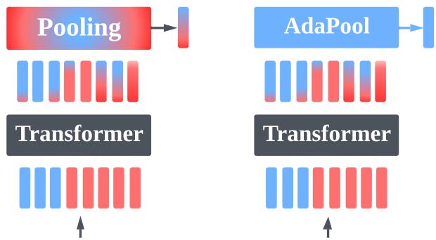
Artificial autonomous systems, such as robots using reinforcement learning (RL) or computer vision models, face the exact same challenge. They are bombarded with sensory inputs. A modern Transformer architecture processes these inputs as a set of vectors (tokens). However, at the end of the processing pipeline, the system often needs to make a single decision: Turn left, Classify as “Cat”, or Grab the object. This requires condensing a large set of output embeddings into a single, actionable representation.

This process is called Pooling.

In non-sequential tasks like vision or RL, practitioners typically resort to standard methods: Average Pooling (taking the mean of all outputs), Max Pooling (taking the maximum value), or using a learned Class Token (CLS). These are often treated as arbitrary design choices.

However, recent research reveals that these standard choices are brittle. They fail catastrophically when the ratio of useful “signal” to irrelevant “noise” in the input changes.

In this post, we dive deep into the paper “Robust Noise Attenuation via Adaptive Pooling of Transformer Outputs.” We will explore why standard pooling methods are mathematically destined to fail under variable noise conditions, and how Adaptive Pooling (AdaPool)—an attention-based aggregation mechanism—provides a theoretically robust solution for autonomous systems.

The Problem: Pooling as Vector Quantization

To understand why pooling matters, we must reframe it. It is not just a dimension-reduction step; it is a compression problem.

Consider an input set of vectors \(\mathbf{X}\). In any given scenario, a subset of these vectors contains information relevant to the task (Signal, \(\mathbf{X}_s\)), and the rest are distractors (Noise, \(\mathbf{X}_\eta\)).

• Signal (\(k\) vectors): Entities or pixels that affect the correct output.
• Noise (\(N-k\) vectors): Background scenery, irrelevant agents, or static.
• SNR: The Signal-to-Noise Ratio is defined as \(k/N\).

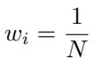
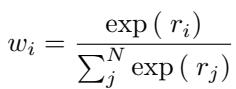
The goal of a global pooling method is to compress the set \(\mathbf{X}\) into a single vector \(\mathbf{x}_c\) that retains as much signal as possible while discarding the noise. We can define a pooling function \(C(\mathbf{X})\) generally as a weighted sum of the inputs:

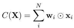
Here, \(\mathbf{w}_i\) represents the weight assigned to each input vector.

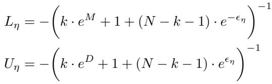
Defining Failure: Signal Loss

How do we measure if a pooling method is working? We borrow concepts from Vector Quantization (VQ). In VQ, the “optimal” compression of a cluster of points is their centroid (the arithmetic mean). Therefore, the optimal representation of our input is the centroid of the signal vectors, ignoring the noise vectors entirely.

We define Signal Loss (\(\mathbb{L}\)) as the Mean Squared Error (MSE) between our pooled output \(\mathbf{x}_c\) and the true signal vectors:

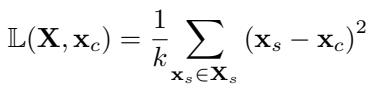
The mathematical goal is simple: Minimize Signal Loss. To achieve zero signal loss, a pooling method must assign weights perfectly:

1. Uniform weight (\(\frac{1}{k}\)) to every signal vector.
2. Zero weight (\(0\)) to every noise vector.

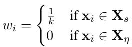
If a pooling method deviates from this weight distribution, it introduces interference. As we will see, standard methods almost always deviate.

The Fragility of Standard Pooling

The paper provides a rigorous analysis of why Average and Max pooling are insufficient for robust systems. They possess “inductive biases” that only work in extreme, specific scenarios.

1. Global Average Pooling (AvgPool)

AvgPool is the default choice for many non-sequential Transformer tasks. It calculates the mean of all output vectors.

Implicitly, this assigns a weight of \(1/N\) to every single vector, regardless of its content.

When does AvgPool work?

AvgPool is only optimal in two rare cases:

1. No Noise: The input set is pure signal (\(\mathbf{X}_\eta = \emptyset\)).
2. Identical Distributions: The average of the noise vectors happens to be exactly the same as the average of the signal vectors.

The Failure Mode

In reality, signal and noise are rarely identically distributed. If you are trying to identify a pedestrian (signal) in a foggy field (noise), the “average” of the fog is not the same as the “average” of the person.

As the amount of noise (\(N\)) increases while the signal (\(k\)) stays fixed, AvgPool dilutes the signal representation. The weight assigned to the signal (\(1/N\)) shrinks toward zero, while the collective weight of the noise grows. AvgPool collapses in low-SNR regimes.

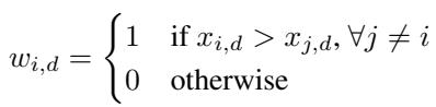
2. Global Max Pooling (MaxPool)

MaxPool takes the maximum value across the feature dimension for every vector.

When does MaxPool work?

MaxPool is extremely selective. It effectively assigns a weight of 1 to the vector with the highest value in a specific feature dimension and 0 to everyone else. It is optimal only if there is exactly one signal vector (\(k=1\)) and that vector contains the maximum value for every feature.

The Failure Mode

MaxPool assumes a “winner-take-all” scenario. If you have multiple signal vectors that need to be aggregated to form a complete picture (e.g., three agents coordinating to lift a box), MaxPool will pick only the most extreme features from them, potentially destroying the relational information. MaxPool tends to perform well when signal is very sparse (finding a needle in a haystack), but fails when the signal is complex and distributed.

The Solution: Adaptive Pooling (AdaPool)

If AvgPool is too democratic (everyone gets a vote) and MaxPool is too autocratic (only the loudest voice counts), we need a method that can adapt its voting system based on the content of the vectors.

The authors propose using the attention mechanism itself as a pooling layer. This is termed AdaPool.

How AdaPool Works

AdaPool uses a standard Key-Query-Value (KQV) attention mechanism, but with a specific setup:

1. Input: The set of vectors \(\mathbf{X}\) serves as the Keys and Values.
2. Query: A single query vector \(\mathbf{x}_q\) is chosen (more on this later).
3. Kernel: A relation function (dot product) measures the similarity between the query and every input vector.

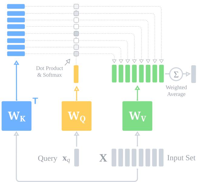
The attention scores determine the weights. A Softmax function normalizes these scores, ensuring they sum to 1.

The Unified Theory of Pooling

One of the paper’s most elegant theoretical contributions is proving that AvgPool and MaxPool are just special cases of AdaPool.

• AvgPool is AdaPool with a Zero Kernel: If the query and key weights are zero matrices, the dot products become zero. \(\exp(0) = 1\). The Softmax divides 1 by \(N\), resulting in \(1/N\) weights—identical to Average Pooling.
• MaxPool is AdaPool at the Limit: If we scale the attention scores by a temperature parameter \(\beta\), as \(\beta \to \infty\), the Softmax function becomes a “hard” max, assigning all weight to the vector with the highest dot product.

This suggests that AdaPool spans the entire spectrum of pooling behaviors. By learning the weights \(W_Q\) and \(W_K\), the network can learn to behave like AvgPool, MaxPool, or anything in between, depending on the current input’s SNR.

The Mathematics of Robustness

Why is AdaPool more robust? It comes down to the Margin.

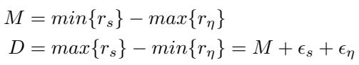
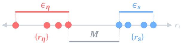
To approximate the optimal quantizer (weights of \(1/k\) for signal, \(0\) for noise), the attention mechanism must create a separation between the relation scores of the signal vectors (\(r_s\)) and the noise vectors (\(r_\eta\)).

We define the “neighborhoods” (spread) of the signal and noise scores:

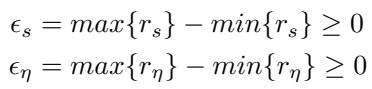
And the Margin (\(M\)) and Distance (\(D\)) between these neighborhoods:

Visualizing this helps intuition:

The authors derive explicit error bounds. They prove that AdaPool can approximate the optimal weights with an error that shrinks as the Margin \(M\) increases.

The Takeaway: As long as the transformer can learn an embedding space where signal vectors are more similar to the query than noise vectors (creating a positive margin \(M\)), AdaPool pushes the weights of noise vectors toward zero exponentially fast.

Choosing the Query Vector

For AdaPool to work, we need a query \(\mathbf{x}_q\).

• Bad idea: Using a fixed learned parameter (like the CLS token). This is static and cannot adapt to rotating or shifting signal distributions.
• Bad idea: Using the average of the inputs. This is corrupted by noise.
• Good idea: Selecting a vector from the signal subset.

In many tasks, we know at least one vector that is likely relevant. In RL, this might be the agent’s own state vector. In Vision, it might be the central patch of the image (assuming the subject is centered). This anchors the attention mechanism, allowing it to “pull” other relevant vectors out of the noise.

Experimental Validation

The theory predicts that standard pooling will fail as SNR fluctuates, while AdaPool should remain stable. The experiments confirm this vividly.

1. Synthetic Supervised Learning

The researchers created a dataset of point sets where they explicitly controlled \(N\) (total points) and \(k\) (signal points needed to find a target centroid). This allows testing across the full SNR spectrum, from 0.01 to 1.0.

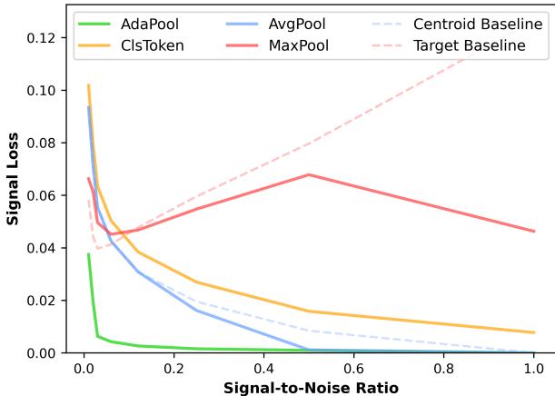
Analysis of Figure 4:

• AvgPool (Blue): Performs well at SNR=1.0 (pure signal) but error skyrockets as noise increases (SNR drops).
• MaxPool (Red): Performs reasonably well at very low SNR (needle in a haystack) but fails as the signal becomes more complex (high SNR).
• AdaPool (Green): Domination. It hugs the bottom of the graph, maintaining near-zero signal loss across almost the entire spectrum. It successfully adapts its strategy.

2. Multi-Agent Reinforcement Learning (MPE)

In the Multi-Particle Environment (MPE), agents must cooperate or compete. The researchers introduced “noise agents”—particles that exist but are irrelevant to the task.

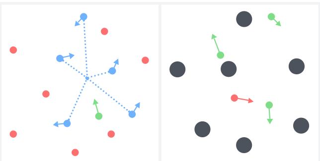
They tested a “Simple Centroid” task (go to the center of signal agents) and a “Predator-Prey” tag game.

Results (Simple Centroid): As the number of signal agents decreased (lowering SNR), standard methods collapsed.

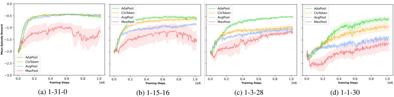
• Plot (c) and (d) represent high-noise scenarios. Look at the Green line (AdaPool). It converges to high rewards while AvgPool and MaxPool struggle significantly. MaxPool is particularly bad here because the task requires aggregating positions from multiple signal agents, which MaxPool cannot do.

Results (Simple Tag): In the tag scenario, they scaled up the number of obstacles (noise).

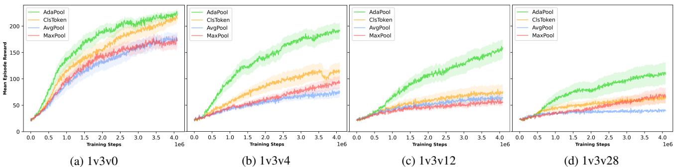
As obstacles increase (moving from left plots to right plots), the performance of AvgPool (Blue) and MaxPool (Red) degrades sharply. AdaPool (Green) maintains the highest win rate, proving it is sample-efficient and robust to visual clutter.

3. Relational Reasoning (BoxWorld)

BoxWorld is a puzzle game requiring complex relational reasoning (keys open locks, which contain other keys). It is visually sparse but logically dense.

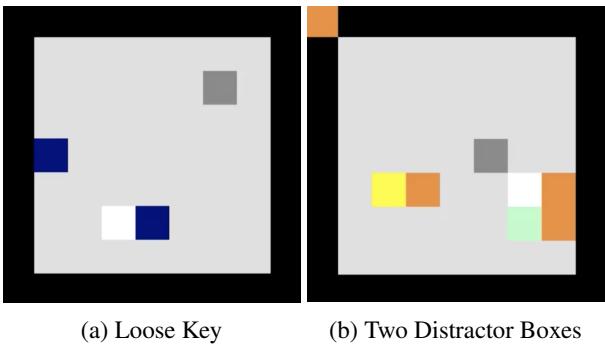
The authors tested two observation types:

1. Entity-based: High signal, low noise.
2. Pixel-based: Massive noise (mostly empty black space).

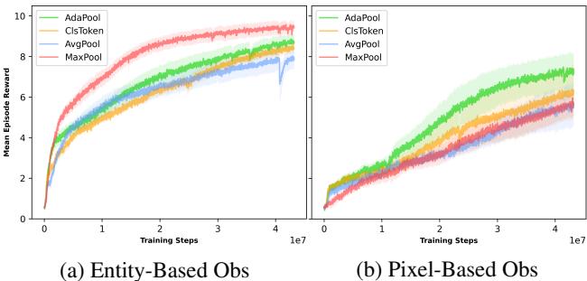
This result is fascinating. In (a) Entity-based, MaxPool (Red) actually learns very fast. Why? Because the “Gem” (goal) is white (pixel value 1.0). MaxPool is biased to find this max value. However, in (b) Pixel-based, the noise overwhelms MaxPool’s naive bias. AdaPool (Green) remains the only consistent performer that solves the puzzle in the high-noise pixel regime.

4. Computer Vision (CIFAR)

Does this apply to real images? They trained Vision Transformers (ViT) on CIFAR-10 and CIFAR-100. The challenge: What is the “Query” for AdaPool in an image? They hypothesized that the central patches of an image usually contain the object of interest.

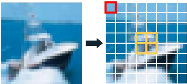
They compared:

• Ada-Corner: Query is a corner patch (likely background/noise).
• Ada-Focal: Query is the center patches (likely signal).
• Ada-Mean: Query is the average of all patches.

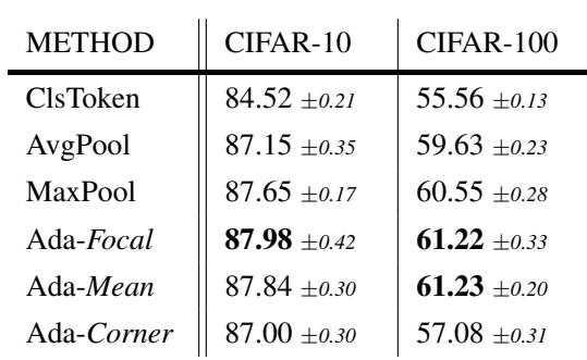
Ada-Focal and Ada-Mean outperformed the standard CLS token and AvgPool. Even Ada-Mean, which uses a noisy query, performed surprisingly well, suggesting that the attention mechanism is robust enough to filter noise even if the query isn’t perfect, provided it captures the general “gist” of the image.

Conclusion

The choice of pooling layer in a Transformer is often an afterthought, but this research shows it is a critical architectural decision.

• AvgPool assumes a clean, balanced world. It fails when noise dominates.
• MaxPool assumes a sparse, simple world. It fails when the signal is complex.
• AdaPool assumes nothing. By leveraging the attention mechanism, it dynamically weights inputs, effectively “learning to pool.”

The authors demonstrated that AdaPool isn’t just an empirical hack; it approximates the mathematically optimal vector quantizer. For students and researchers designing autonomous systems—whether they are robots navigating cluttered rooms or agents playing complex games—replacing that final mean() with an adaptive attention layer might be the simplest way to significantly boost robustness.