](https://deep-paper.org/en/paper/2507.02119/images/cover.png)
If you have ever trained a large neural network, you know the process can feel a bit like alchemy. You mix a dataset, an architecture, and an optimizer, staring at the loss curve as it (hopefully) goes down. We have developed “Scaling Laws”—empirical power laws that predict the final performance of a model based on its size and compute budget. But the path the model takes to get there—the training dynamics—has largely remained a messy, unpredictable black box.
Until now.
In a fascinating new paper, Scaling Collapse Reveals Universal Dynamics in Compute-Optimally Trained Neural Networks, researchers from NYU and Google DeepMind have uncovered a hidden symmetry in the chaos of training. They demonstrate that if you train models “compute-optimally” (balancing model size and training duration efficiently), the loss curves of tiny models and massive models are effectively identical.
This phenomenon, which they call Scaling Collapse, suggests that despite the complexity of modern AI, there is a simple, universal “shape” to learning. Even more surprisingly, under certain conditions, this universality becomes so precise that it breaks the standard noise floor of experiments—a phenomenon dubbed Supercollapse.
In this post, we will unpack the mathematics behind this universality, explore the simple model that predicts it, and discuss why this matters for the future of scaling deep learning.
The Quest for Compute Optimality
Before understanding the collapse, we need to understand the setup. The researchers focused on compute-optimal training. This concept, popularized by the “Chinchilla” paper (Hoffmann et al., 2022), asks a simple question: For a given budget of FLOPs (computational operations), what is the best allocation of model parameters (\(p\)) and training tokens (\(t\))?
If you have a huge budget, you shouldn’t just train a small model for a trillion years, nor should you train a gargantuan model for just one epoch. There is a “sweet spot” balance where the model size and dataset size grow together.
The researchers trained a “scaling ladder”—a sequence of Transformers and MLPs of increasing widths—where each model was trained for its specific compute-optimal horizon \(t^*(p)\).
The Discovery: Universal Loss Curves
When you plot the raw loss curves of these different models, they look distinct. Larger models start with different losses and converge to lower values. However, the authors discovered that these curves are actually shadows of a single, universal trajectory.
To see this, they applied a normalization to the loss curves. They defined a normalized loss curve \(\ell(x, p, \omega)\) by rescaling the time and the loss:
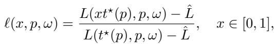
Here:
- \(x\) is the normalized compute (ranging from 0 to 1), representing the fraction of the training budget used.
- \(\hat{L}\) is the irreducible loss (the lowest possible loss, e.g., inherent entropy in the data).
- The denominator normalizes the progress relative to the final achieved loss.
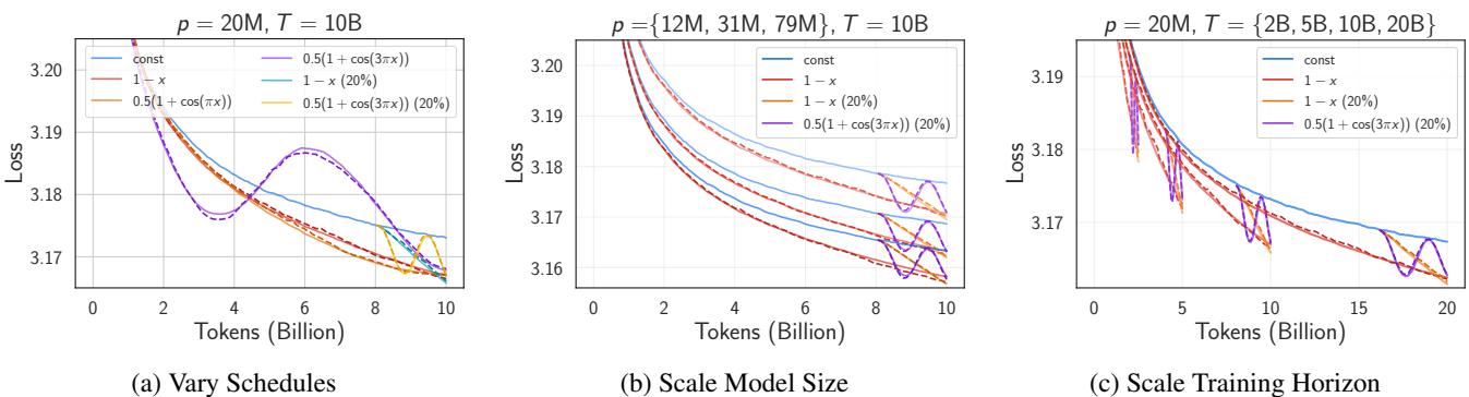
When the researchers applied this transformation to models of vastly different sizes (from 10M to 80M parameters), something remarkable happened.
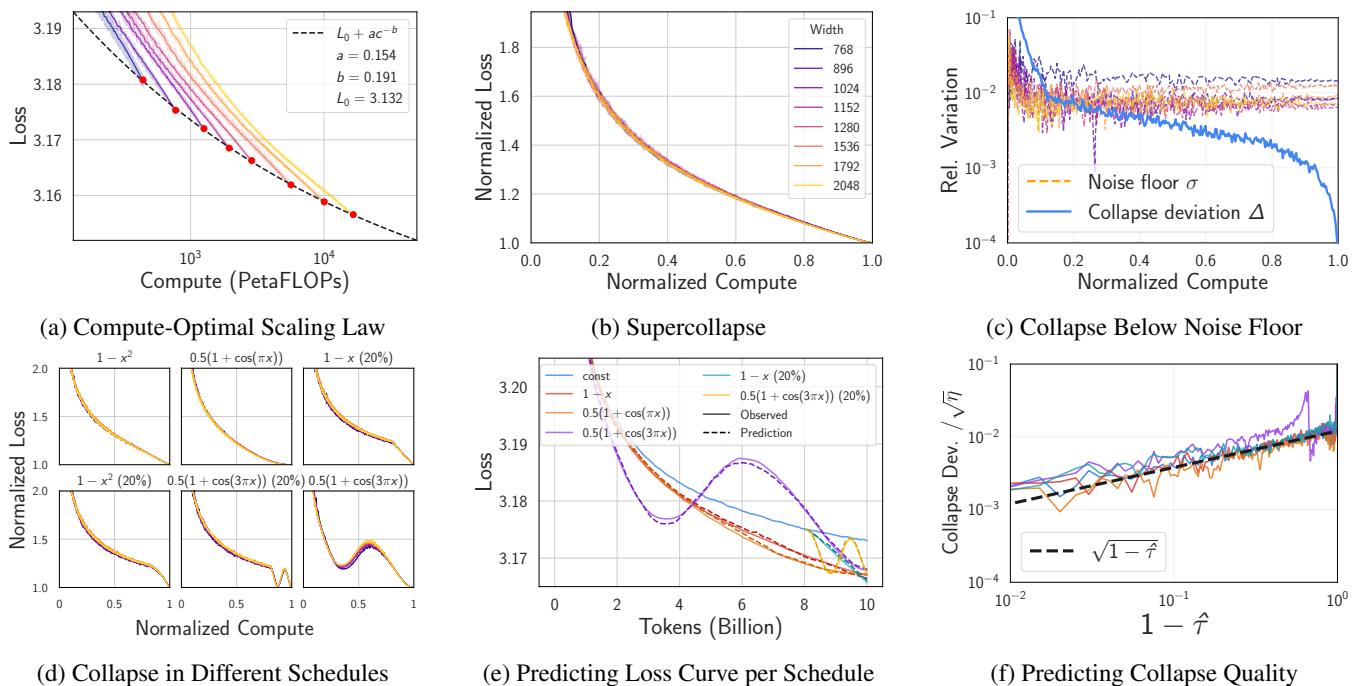
As shown in Figure 1(b) above, the curves collapsed onto each other. A small model at 50% of its training budget behaves statistically identically to a large model at 50% of its budget. This is Scaling Collapse. It implies that the rate of relative progress is invariant to scale.
The Role of Irreducible Loss
A crucial detail in this normalization is subtracting \(\hat{L}\), the irreducible loss. If you try to normalize without accounting for the noise inherent in the dataset (the “entropy floor”), the collapse fails.
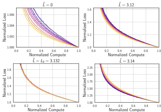
Figure 2 illustrates this sensitivity. The collapse is sharpest when \(\hat{L}\) matches the estimated irreducible loss \(L_0\). This sensitivity is actually useful—it acts as a sanity check for whether we have correctly estimated the fundamental limits of the dataset.
Enter “Supercollapse”
The collapse is interesting enough with a constant learning rate, but modern training uses schedules (like linear decay or cosine annealing) to lower the learning rate as training progresses. When the researchers analyzed these schedules, they found something bizarre.
With learning rate decay, the normalized curves from different models matched each other better than two random seeds of the same model match each other.
To quantify this, they defined the Collapse Deviation \(\Delta(x)\) (the difference between models) and compared it to the Noise Floor \(\sigma(x, p)\) (the difference between random seeds).

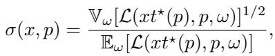
In a standard experiment, you would expect the variation between different model sizes (\(\Delta\)) to be larger, or at best equal to, the random noise (\(\sigma\)).
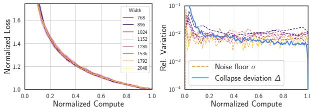
With a constant learning rate (Figure 3), \(\Delta\) is roughly equal to \(\sigma\). But look back at Figure 1(c). Under a decay schedule, the blue line (\(\Delta\)) drops below the orange line (\(\sigma\)).
This is Supercollapse. It implies that the normalized dynamics of compute-optimal models are incredibly rigid, constrained by a universal law that suppresses variance as the learning rate drops.
Explaining the Phenomenon
Why does this happen? The authors provide a two-part theoretical explanation: one based on power laws, and one based on the noise dynamics of Stochastic Gradient Descent (SGD).
1. The Power-Law Connection
Empirically, neural scaling laws often follow a sum of power laws:
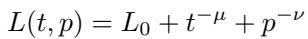
In this equation, \(t^{-\mu}\) represents the error due to limited training time, and \(p^{-\nu}\) represents the error due to limited model size.
The researchers proved mathematically that if you solve for the optimal compute budget, you force a balance between these two terms:
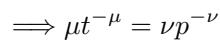
When you plug this balance back into the loss equation and normalize it, the dependency on \(p\) (model size) cancels out entirely:
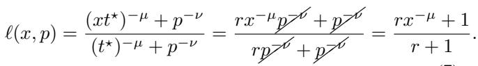
The result on the right side depends only on \(x\) (time) and constants—\(p\) has disappeared. This explains why the curves collapse: Compute optimality forces the finite-width error and finite-time error to scale in lockstep.
2. A Simple Model of SGD Noise
The power-law explanation works for constant learning rates, but it fails to capture the complex shapes of loss curves under Cosine or Linear decay schedules. To explain Supercollapse, the authors modeled the training as a deterministic path plus noise injected by SGD.
They utilized a linearized model of learning dynamics. Surprisingly, they found that the change in loss due to a specific learning rate schedule could be predicted by a simple equation:
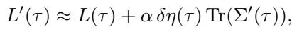
Here, the loss \(L'\) is the original loss plus a term depending on the change in learning rate \(\delta \eta\) and the Trace of the Gradient Covariance (\(\text{Tr}(\Sigma')\)). This trace measures the magnitude of the noise in the gradients.
This simple model is shockingly effective.
As shown in Figure 6, this theoretical model (dashed lines) accurately predicts the real training curves of Transformers on CIFAR-5M (solid lines) across various schedules and model sizes.
3. Why Supercollapse? (Variance Reduction)
The theoretical model also explains why Supercollapse beats the noise floor. It comes down to correlations.
When we normalize the loss curve, we divide the current loss by the final loss of that specific run. Because SGD noise is correlated over time, a run that is “unlucky” (higher loss) in the middle of training is likely to be “unlucky” at the end. By dividing by the final loss, we are essentially using the end of training as a control variate.
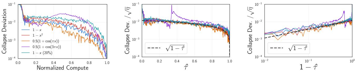
Figure 8 confirms this. The variance of the collapsed curve decreases as the learning rate \(\eta\) decays. The scaling follows \(\sqrt{\eta(1-\hat{\tau})}\). As the learning rate drops to zero, the correlated noise cancels out almost perfectly, driving the collapse deviation toward zero.
Practical Utility: A Diagnostic Tool
Beyond the theoretical beauty, Supercollapse is a powerful tool for AI engineers. Because the collapse is so precise, it acts as a sensitive detector for “bad” scaling.
If you scale your model width but fail to scale your hyperparameters (like initialization or learning rate) correctly, or if your data exponent is wrong, the collapse will break.
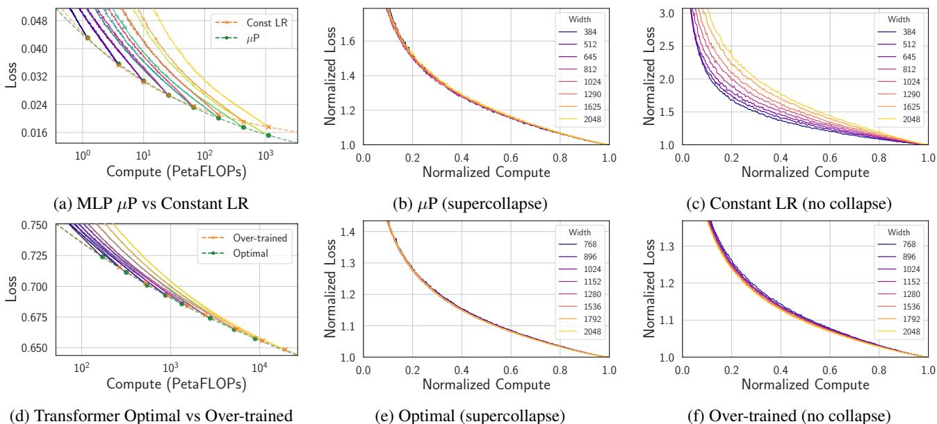
In Figure 4, we see two examples of failure:
- Top Row: Using a constant learning rate across models (instead of the correct \(\mu P\) parameterization) shatters the collapse.
- Bottom Row: Using a suboptimal data exponent (\(\gamma=1.2\) instead of \(1.02\)) causes the curves to drift apart.
This means you can use Scaling Collapse to tune your scaling laws. Instead of training models to completion and fitting a curve to the final points (which is noisy), you can tune your hyperparameters to maximize the tightness of the collapse throughout the entire training trajectory.
Conclusion
The paper “Scaling Collapse Reveals Universal Dynamics” provides a compelling glimpse into the underlying physics of deep learning. It suggests that training large models is not just a chaotic descent down a loss landscape, but a structured, predictable process governed by universal dynamics.
Key takeaways for students and practitioners:
- Universal Shape: Compute-optimally trained models follow a single, universal learning curve when normalized.
- Supercollapse: Learning rate decay suppresses variance so effectively that normalized curves across scales match better than random seeds of the same scale.
- Diagnostic Power: If your loss curves don’t collapse, your scaling strategy (hyperparameters or data mix) is likely suboptimal.
By focusing on the dynamics of the entire loss curve rather than just the final number, we gain a much richer understanding of how neural networks scale—paving the way for more efficient and robust training of the next generation of foundation models.