In the rapidly evolving world of artificial intelligence, a common assumption dictates the rules of the game: if you want a model to excel at a specific task, you must train it on a massive amount of specific data. If you want to diagnose diseases from 3D MRI scans, the conventional wisdom says you need to build a complex 3D neural network and feed it thousands of annotated medical volumes.

But what if that assumption is wrong?

What if you could take a general-purpose vision model—one trained on pictures of dogs, landscapes, and cars—and use it to analyze complex 3D medical scans with state-of-the-art accuracy, without performing any training at all?

This is the premise behind Raptor (Random Planar Tensor Reduction), a groundbreaking technique introduced in a recent research paper. Raptor challenges the “data-hungry” status quo of medical AI. By cleverly combining 2D foundation models with a mathematical concept called random projections, Raptor generates embeddings for 3D volumes that are lightweight, scalable, and surprisingly more effective than models trained specifically on medical data.

In this deep dive, we will explore how Raptor works, the mathematics that makes it possible, and why it might represent a paradigm shift for AI in resource-constrained fields like healthcare.

The Problem: The Curse of Dimensionality in 3D

To understand why Raptor is such a breakthrough, we first need to look at the hurdles facing 3D medical imaging analysis.

Medical data, such as Magnetic Resonance Imaging (MRI) or Computed Tomography (CT) scans, are volumetric. Unlike a 2D JPEG image which is a grid of pixels, a medical volume is a grid of voxels (volumetric pixels). While a standard image might be \(256 \times 256\) pixels, a medical volume is \(256 \times 256 \times 256\).

This added dimension introduces a massive computational penalty.

1. Computational Cost: Processing 3D data requires architectures (like 3D Convolutional Neural Networks or 3D Transformers) that incur cubic computational costs. The memory requirements explode, often requiring expensive, specialized hardware (like clusters of H100 GPUs) that is out of reach for many university labs and hospitals.
2. Data Scarcity: Modern AI thrives on scale. We have datasets with billions of 2D images (like the data used to train DINOv2 or CLIP). In contrast, the largest public 3D medical datasets contain perhaps 100,000 to 160,000 volumes. This is several orders of magnitude smaller than what is needed to train “foundation models” from scratch effectively.

Because of these limitations, researchers have struggled to scale large models for medical volumes. Existing state-of-the-art (SOTA) methods like SuPreM, MISFM, or VoCo try to solve this by pretraining on available medical datasets, but they still require significant compute to train and fine-tune.

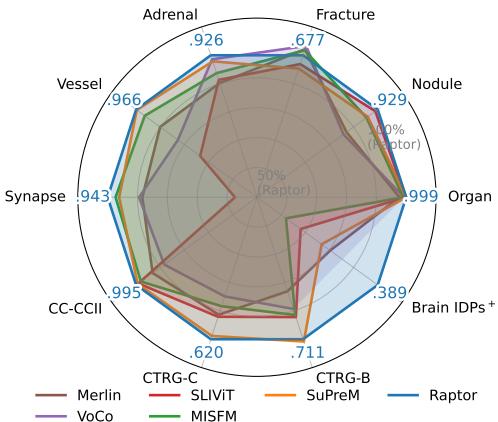
Enter Raptor. As shown in the radar chart below, this new method outperforms these specialized medical models across a wide variety of tasks, from organ classification to nodule detection, without ever “seeing” a medical volume during a training phase.

The Core Concept: 2D Models in a 3D World

The insight driving Raptor is that we don’t necessarily need a 3D brain to understand a 3D object. Just as an architect understands a building by looking at floor plans and elevation drawings, an AI can understand a volume by analyzing its 2D cross-sections.

Furthermore, we already possess incredibly powerful 2D “eyes.” Foundation models like DINOv2 (a Vision Transformer trained by Meta) have seen billions of images. They have learned to identify edges, textures, shapes, and semantic relationships. Raptor posits that these features are universal. A curve is a curve, whether it’s on the fender of a sports car or the edge of a kidney in a CT scan.

The Raptor Pipeline

The Raptor workflow is an exercise in elegance and efficiency. It avoids training a neural network entirely. Instead, it acts as a feature extraction pipeline. Let’s break down the architecture visualized in the figure below.

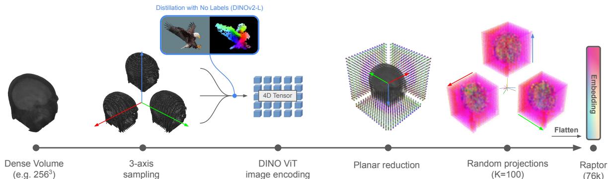
Step 1: 3-Axis Volume Sampling

A dense 3D volume is difficult to process all at once. Raptor starts by slicing the volume along three orthogonal axes:

• Axial: Top-down view (like looking down at the head).
• Coronal: Front-to-back view (like looking at a face).
• Sagittal: Side view (like a profile).

By taking slices from these three perspectives, the method captures the geometry of the internal structures without needing 3D convolutions. This is often referred to as a “tri-planar” approach.

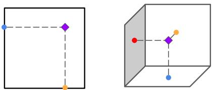
To visualize why looking at these three planes is sufficient to reconstruct 3D information, consider the triangulation principle shown below. If you know where a feature lies on the “floor” (axial) and the “wall” (coronal), you can pinpoint its location in 3D space.

Step 2: Feature Extraction with DINOv2

Once the volume is sliced, each 2D image is fed into a frozen DINOv2-Large image encoder.

“Frozen” is the key word here. The weights of this neural network are never updated. Raptor uses the model exactly as it was downloaded. The model outputs a set of feature tokens (vectors that represent visual information) for patches of the image.

However, this creates a new problem: Explosion of Data. If you take a \(256^3\) volume and extract deep features for every slice, you end up with a tensor that is massive—potentially larger than the original volume itself. Storing these raw features for a dataset of 100,000 volumes would require dozens of terabytes. We need a way to compress this information without losing the semantic meaning.

Step 3: Random Planar Tensor Reduction

This is the main contribution of the paper. How do you compress a massive tensor of features into a small, usable vector?

Raptor employs a two-step reduction strategy:

1. Axial Aggregation: For a specific axis (say, Axial), Raptor takes the average of the features across all slices. This collapses the depth dimension. You might think averaging slices would destroy information, blurring distinct organs together. However, because medical anatomy changes relatively smoothly through space, the aggregate statistics remain highly informative.
2. Random Projection: Even after averaging, the feature vectors are high-dimensional. To shrink them further, Raptor multiplies the feature vector by a Random Matrix (\(R\)).

The mathematical operation looks like this:

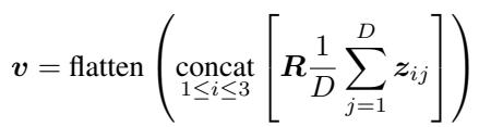
Here, \(z_{ij}\) represents the features from the vision transformer, and \(R\) is a matrix filled with random numbers drawn from a normal distribution.

Wait, Random Numbers?

It seems counter-intuitive. How can multiplying your carefully extracted features by a matrix of random noise be helpful?

This relies on the Johnson-Lindenstrauss (JL) Lemma. In simple terms, the JL Lemma states that points in a high-dimensional space can be projected into a lower-dimensional space while approximately preserving the distances between them.

If two medical scans are “semantically far apart” (e.g., one shows a healthy lung, one shows a tumor) in the high-dimensional feature space of DINOv2, they will remain “far apart” after being multiplied by the random matrix. If they are similar, they will remain close.

This allows Raptor to compress the data massively—reducing the footprint by over 90%—while keeping the essential “fingerprint” of the volume intact. The researchers found that using a projection dimension (\(K\)) of just 100 was enough to achieve state-of-the-art results.

Experimental Dominance

The researchers benchmarked Raptor against the heaviest hitters in the field of medical AI. The baselines included models like SuPreM and MISFM, which were pretrained on tens of thousands of medical volumes using expensive GPUs.

The results were striking. Raptor didn’t just match these models; it consistently beat them.

Classification Performance

On the 3D Medical MNIST benchmark (a standard collection of datasets for classifying medical images), Raptor achieved the highest accuracy in 6 out of 9 datasets. When comparing the area under the curve (AUROC), a metric of classification robustness, Raptor was often superior.

Specifically, compared to SuPreM (a model explicitly trained on 5K CT volumes), Raptor improved metrics by an average of +2%. Against SLIViT (another pretrained model), the improvement jumped to +13%.

Efficiency vs. Accuracy

One of the most compelling arguments for Raptor is its efficiency. The plot below compares the accuracy (AUROC) of different models against their embedding size in memory.

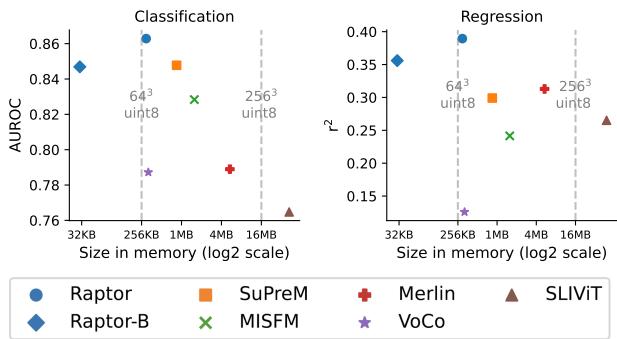
Look at the position of the blue circles (Raptor). They reside in the top-left quadrant, which is the “sweet spot”: high accuracy and low memory usage.

• Raptor-B (Base): Even when using a tiny projection size (\(K=10\)), resulting in a massive compression, the model (labeled Raptor-B) still competes with or beats fully trained models like SuPreM and Merlin (orange and red markers), while using a fraction of the memory.

Few-Shot Learning: Doing More with Less

In medical fields, getting labeled data is expensive. A radiologist’s time is valuable, so we often only have 10 or 20 labeled scans for a specific rare disease.

Raptor excels in this “data-scarce” environment. Because the embeddings are already rich with semantic information from the foundation model, a simple classifier trained on top of them needs very few examples to learn.

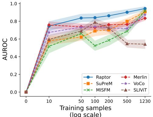
The graph above shows the performance on the Synapse dataset. With only 10 training samples, Raptor (the blue line) achieves nearly 80% of its maximum performance. Other models like MISFM (green) or SLIViT (brown) struggle significantly when data is limited, often performing little better than random guessing until they see hundreds of examples.

Why Does It Work? The Science of Smoothness

The success of Raptor relies on the assumption that medical volumes are “smooth.” This means that if you look at slice \(N\) and slice \(N+1\), they look very similar. The features don’t jump erratically.

The researchers analyzed this by calculating a value, \(\alpha_j\), which estimates the alignment between consecutive slices in the feature space.

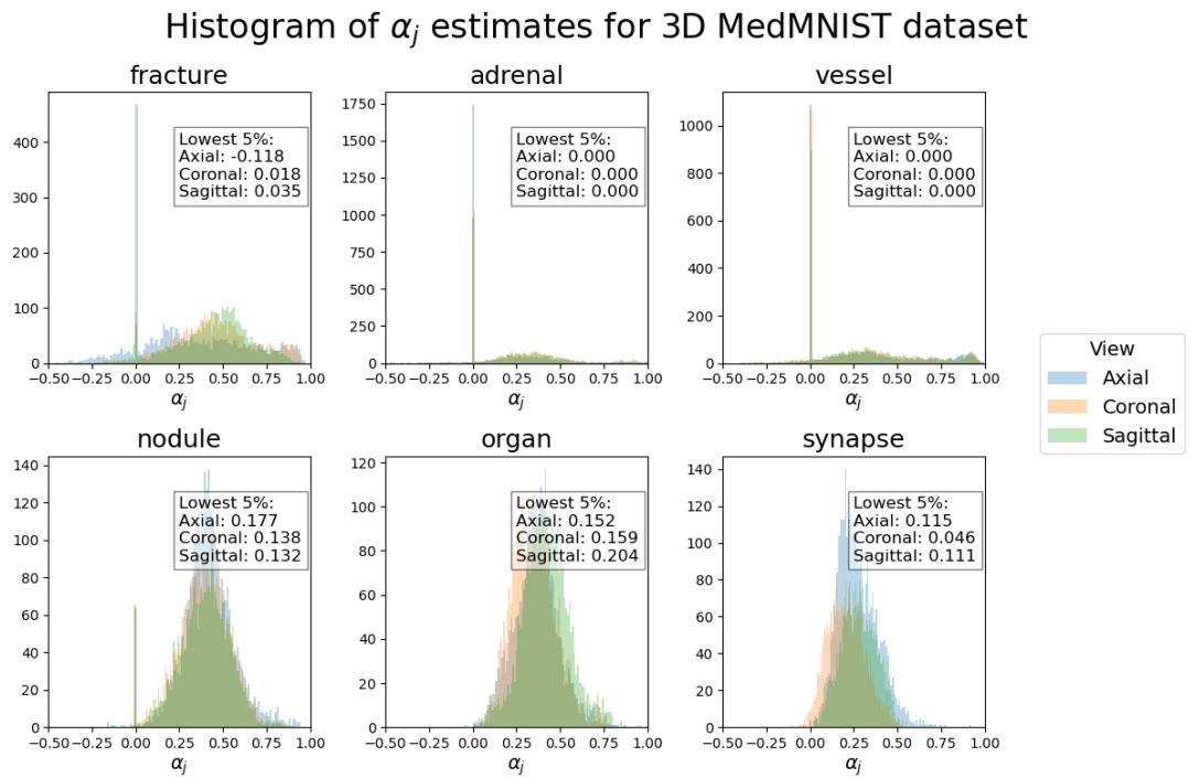
In this histogram, positive values (to the right) indicate good alignment—meaning the features change smoothly. Most datasets (like Organ, Nodule, and Vessel) show strong positive alignment, explaining why Raptor works so well.

However, looking at the Fracture dataset (top left), we see a wider spread, with some values dipping below zero. Fractures are, by definition, discontinuities—breaks in the bone structure. This lack of smoothness makes averaging slices slightly less effective, which aligns with the experimental results where Raptor’s lead on the Fracture dataset was smaller than on others. This honest analysis highlights both the strength of the method and its theoretical boundaries.

Conclusion: A “Train-Free” Future?

Raptor represents a significant step toward democratizing medical AI. By removing the need for computationally expensive pretraining, it allows researchers with standard consumer hardware (like a single gaming GPU) to achieve state-of-the-art results.

The implications are broad:

1. Accessibility: You don’t need a data center to build a world-class medical diagnostic tool.
2. Agility: As general vision models improve (e.g., DINOv3 or newer architectures), Raptor improves instantly. You simply swap out the frozen encoder.
3. Data Privacy: Since no training is required on the sensitive medical volumes themselves to generate the embeddings, the barrier to entry regarding patient privacy is lowered for the feature extraction phase.

Raptor proves that sometimes, the best way to solve a complex 3D problem isn’t to build a bigger, more complex 3D model. Sometimes, it’s better to look at the problem from a few different angles—literally—and let the math do the rest.