](https://deep-paper.org/en/paper/2507.09177/images/cover.png)
Imagine you are teaching a robot to make coffee. After weeks of training, it finally masters the art of grinding beans and pouring water. Next, you teach it to load the dishwasher. It learns quickly, but when you ask it to make coffee again, it stares blankly at the machine. It has completely overwritten its “coffee-making” neurons with “dishwasher-loading” neurons.
This phenomenon is known as catastrophic forgetting, and it is the Achilles’ heel of Artificial Intelligence.
In standard Deep Reinforcement Learning (RL), agents are great at mastering a single task. But in Continual Reinforcement Learning (CRL)—where an agent must learn a sequence of tasks one after another—standard methods fail. They suffer from stability-plasticity dilemmas: if the brain is too plastic, it overwrites old memories (forgetting); if it’s too stable, it can’t learn new things.
In this post, we will dive into a fascinating paper titled “Continual Reinforcement Learning by Planning with Online World Models” by Liu et al. The researchers propose a shift in perspective: instead of memorizing how to act (policies), the agent should focus on learning how the world works (world models) using a method that mathematically guarantees it won’t forget.
The Problem: Task IDs and Conflicting Realities
To understand why CRL is so hard, we first need to look at how researchers have traditionally tried to solve it. A common “cheat” in this field is using Task IDs. When the robot switches from coffee to dishes, the environment tells the robot: “Switching to Task 2.” The robot then loads a different set of neural weights or uses a specific part of its brain allocated for Task 2.
But in the real world, life doesn’t give us Task IDs. A robot moving through a kitchen just sees a continuous stream of sensory data.
Furthermore, many previous approaches treat different tasks as having entirely separate physical dynamics. The authors highlight this issue using a concept called Unified Dynamics.
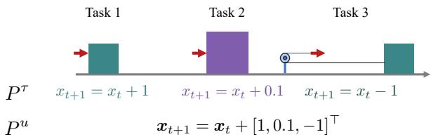
As shown in Figure 1, if we treat tasks separately (\(P^\tau\)), the same action in the same state might produce different outcomes depending on the “Task ID.” This forces the agent to learn conflicting rules. However, in reality, physics is consistent (\(P^u\)). Gravity doesn’t change just because you decided to switch tasks.
The authors propose an Online Agent (OA). This agent assumes there is one unified world model. It learns this model incrementally and uses it to plan its actions.
The Solution: The Online Agent (OA)
The Online Agent is built on three pillars:
- Online World Model Learning: Learning the physics of the environment in real-time.
- No-Regret Updates: A mathematical way to update the model that ensures optimal learning over time.
- Planning: Using the learned model to simulate futures and choose the best action.
1. The Architecture: Shallow and Wide
Deep Neural Networks (DNNs) are the standard for RL, but they are terrible at online learning. If you update a DNN on a single new data point, it often drastically changes its weights, destroying previous knowledge. To fix this, you usually need a “replay buffer” to constantly remind the network of old data. This is slow and memory-intensive.
The authors instead use a Follow-The-Leader (FTL) shallow model. Instead of a deep network, they use a non-linear feature extractor followed by a single linear layer.
- The Input: State (\(s\)) and Action (\(a\)).
- The Feature Extractor (\(\phi\)): They use a “Locality Sensitive Sparse Encoding.” Imagine a massive, high-dimensional grid. Any specific state-action pair activates only a few specific “neurons” in this grid. This works like a static, random projection that makes the data separable.
- The Linear Layer (\(W\)): This maps the features to the next state (\(s'\)).
Because the last layer is linear, the “best” weights can be calculated mathematically using a closed-form equation, rather than imperfectly estimated via Gradient Descent.
2. The Learning Algorithm: Sparse Recursive Updates
The magic happens in how the agent updates its understanding of the world. Since the agent uses a linear model on top of sparse features, it can use a Recursive Least Squares approach.
This allows the agent to update its model instantly after every single step in the environment, without needing to retrain on old data to prevent forgetting. The math ensures that the new update respects all previous history.
The update rule for the weights (\(W\)) looks like this:
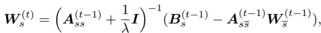
Here, \(\boldsymbol{A}\) represents the accumulated covariance of all data seen so far (the history), and \(\boldsymbol{B}\) represents the targets. By maintaining these matrices, the agent has a “perfect memory” of the statistics of the past, compacted into a matrix, rather than storing millions of raw replay frames.
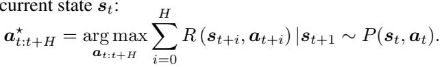
3. Acting via Planning
Once the agent has a working model of the world (\(P(s'|s,a)\)), it doesn’t need to learn a policy network (which takes a long time). Instead, it plans.
The agent looks at the current state, uses its world model to hallucinate thousands of different action sequences, and evaluates which one yields the highest reward. This is done using the Cross-Entropy Method (CEM), a powerful evolutionary algorithm for optimization.
By separating the dynamics (which are shared across all tasks) from the reward (which changes per task), the agent becomes extremely adaptable. When the task switches, the agent simply swaps the reward function it’s planning for, while keeping all the physical knowledge it has accumulated.
Theoretical Guarantee: No-Regret Learning
One of the strongest contributions of this paper is the theoretical proof. In Deep RL, we often cross our fingers and hope the network converges. Here, the authors prove a Regret Bound.
Regret is the difference between the total error the agent actually made during learning and the error the best possible offline model (one that saw all the data at once) would have made.
The authors prove that their sparse online update rule achieves a regret of:
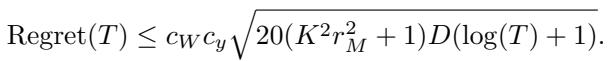
Simply put, this equation means the agent’s performance gap (compared to a perfect oracle) shrinks rapidly over time (\(O(\sqrt{\log T})\)). It guarantees that the agent is efficiently converging to the true world physics without catastrophic forgetting.
Continual Bench: A Better Testing Ground
To test their agent, the authors realized existing benchmarks were flawed. Many benchmarks, like “Continual-World,” effectively “teleport” objects or change physical constraints between tasks in ways that make a unified physics model impossible.
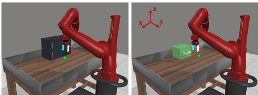
As seen in Figure 2, if an environment uses the same input coordinates for a door handle (circular motion) and a drawer handle (linear motion), a single world model will be confused. It’s a “physical conflict.”
To solve this, the authors introduced Continual Bench.
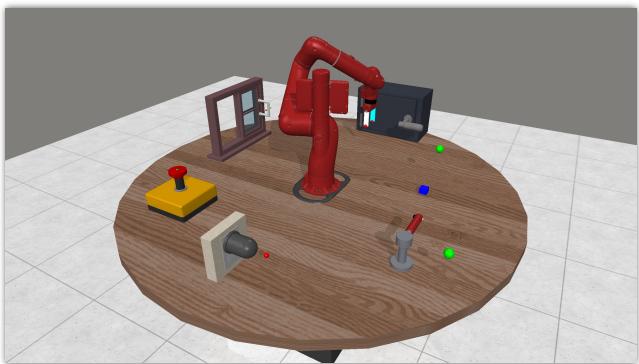
In Continual Bench (Figure 3), tasks are arranged spatially. The robot is in the center, and the tasks (window, door, faucet, etc.) are placed around it. This creates a consistent physical world where “Unified Dynamics” actually exist. The robot can learn the physics of the window, turn around, learn the faucet, and still remember how the window works because the window is still there, governed by the same laws of physics.
Experimental Results
The researchers compared their Online Agent (OA) against several strong baselines:
- Fine-tuning: A standard deep model that just keeps training (expected to forget).
- EWC, SI, PackNet: Popular Continual Learning methods designed to protect weights from changing too much.
- Coreset: A method that keeps a small buffer of old data to replay.
- Perfect Memory: An idealized baseline that stores everything and retrains constantly (computational cheating).
1. Performance Over Time
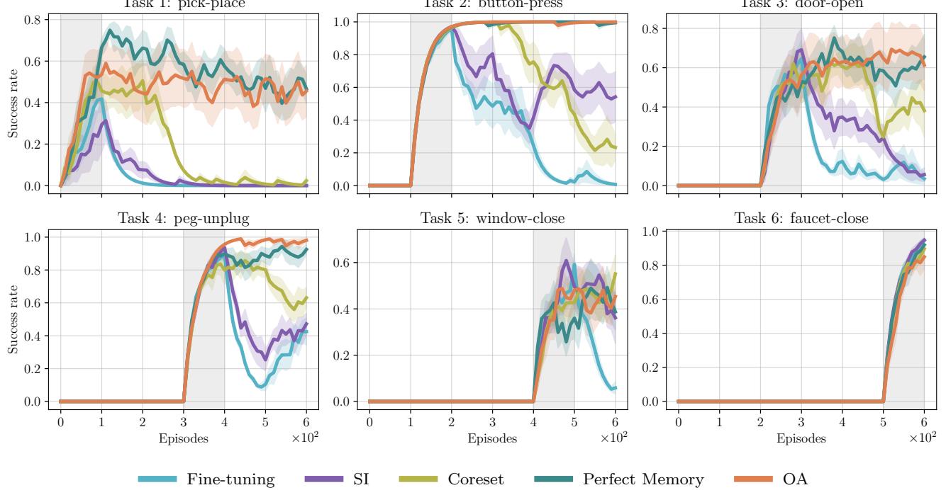
Figure 5 tells the main story. Look at the orange line (OA).
- When a new task starts (grey shaded area), OA learns it quickly.
- Crucially, after the task finishes and the robot moves to the next one, the orange line stays high.
- Compare this to Fine-tuning (cyan) or SI (purple), which often drop to zero success on old tasks immediately after switching.
2. Average Performance and Regret
To summarize performance, we can look at the Average Performance (AP) across all tasks seen so far.
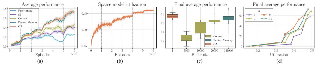
In Figure 6(a), the Online Agent (orange) climbs steadily, matching the “Perfect Memory” baseline (dark teal). This confirms that the lightweight, recursive update is just as effective as storing the entire dataset, but infinitely more efficient.
We can also quantify the Regret—the area between the agent’s performance and a perfect performance (Oracle).
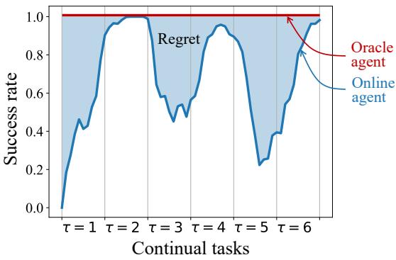
Using the metric defined in Figure 4, the OA achieved significantly lower regret than model-free baselines and matched the best model-based baselines, proving it learns faster and retains more.
3. Does it actually remember the physics?
Finally, the authors checked the internal error of the world models. Did the neural networks actually remember the physics, or did they just get lucky?
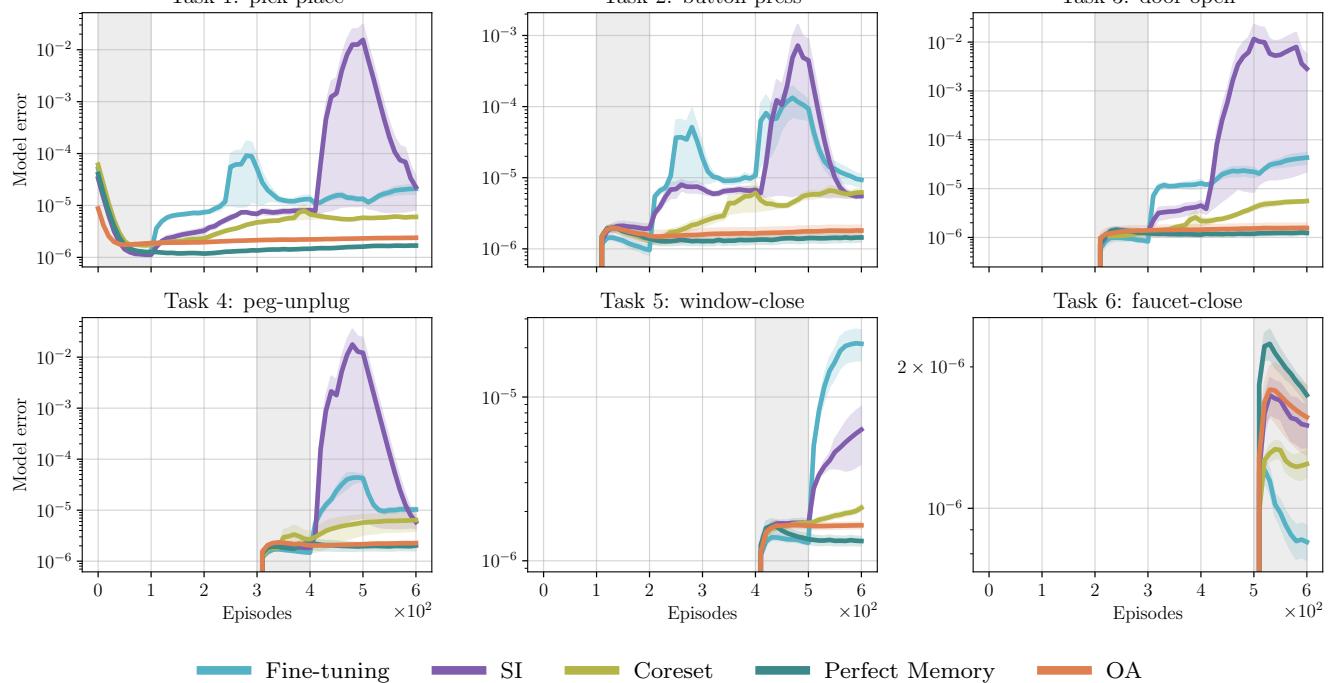
Figure 8 is perhaps the most damning for standard deep learning methods. Look at Task 1 (Pick-Place).
- The OA (orange) maintains a flat, low error line forever.
- SI (purple) and Fine-tuning (cyan) show massive spikes in error for Task 1 as soon as they start learning Task 2, 3, or 4. They are literally forgetting the physics of the first object.
Conclusion
The “Online Agent” paper presents a compelling argument for the future of robotic learning. By moving away from “black box” neural networks that memorize policies, and toward model-based agents with mathematically grounded update rules, we can create systems that truly learn.
The key takeaways are:
- Shared Dynamics: Real-world continual learning relies on the fact that physics doesn’t change.
- Online Updates: Recursive, closed-form updates (like FTL) prevent catastrophic forgetting naturally, without complex auxiliary losses.
- Planning is Robust: If you know how the world works, you can solve new tasks zero-shot simply by changing your goal.
This approach brings us one step closer to generalist robots that can learn to load the dishwasher without forgetting how to make our morning coffee.