](https://deep-paper.org/en/paper/2507.09897/images/cover.png)
Introduction
One of the most profound mysteries in deep learning is the phenomenon of generalization. We typically understand generalization through the lens of interpolation: if a neural network sees enough training examples (dots on a graph), it learns a smooth curve that connects them, allowing it to predict values for points situated between the training examples.
However, in certain settings, neural networks exhibit a behavior that defies this interpolation-based explanation. They learn to extrapolate. They can handle inputs far beyond the bounds of their training data—sometimes infinitely so. When a network trained on short sequences suddenly solves a task for sequences thousands of times longer, it implies the network hasn’t just fitted a curve; it has discovered an underlying algorithm.
How does a process as simple as gradient descent—which only seeks to minimize error on specific training data—stumble upon a general-purpose algorithm?
This post dives deep into a recent study that dissects this phenomenon using the Streaming Parity Task. By analyzing the learning dynamics of Recurrent Neural Networks (RNNs), we will explore a theoretical framework that models neural representations as interacting particles. We will see how “implicit state mergers” drive the network from rote memorization to algorithmic perfection.
The Problem: Infinite Generalization from Finite Data
To study algorithmic learning, we need a task that cannot be solved by simple approximation. Enter the Streaming Parity Task.
The task is simple but non-linear: Given a stream of binary digits (0s and 1s), the network must output 0 if the total number of ones seen so far is even, and 1 if it is odd. This is equivalent to computing the cumulative XOR of the stream.
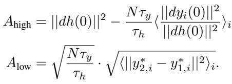
Here is the crucial setup: The researchers trained an RNN on sequences of a finite length (e.g., up to length 10). They then tested it on sequences of length 10,000.
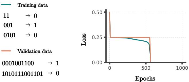
As shown in Figure 1, the network achieves near-zero loss on sequences orders of magnitude longer than the training set. Since the “long sequence” domain is completely disjoint from the “short sequence” domain, interpolation is impossible. The network must have learned the precise logic of parity.
Background: RNNs and Automata
To understand how the network learns this, we need to look inside the “black box.” A standard interpretation of RNNs involves dynamical systems, but for algorithmic tasks, a more powerful lens is Automata Theory.
The Target Algorithm: A DFA
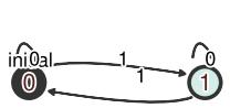
The streaming parity task can be perfectly described by a Deterministic Finite Automaton (DFA) with just two states.
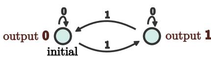
In this DFA (Figure 2), the system effectively has a 1-bit memory: “Even” (Output 0) or “Odd” (Output 1).
- If it sees a
0, it stays in the current state. - If it sees a
1, it transitions to the other state.
Extracting Automata from Neural Networks
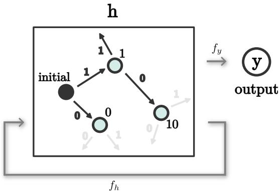
An RNN operates in continuous vector space, not discrete states. Its defining equations are:
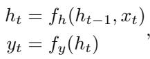
Here, \(h_t\) is the high-dimensional hidden state vector. To check if the RNN has learned the DFA, we treat the hidden vectors \(h_t\) as “states.” If the network is solving the task algorithmically, the infinite number of possible hidden vectors should cluster into a finite set of functional states.
The researchers used a technique to extract these automata. They pass sequences through the network and observe the resulting hidden vectors. If two different sequences result in hidden vectors that are very close to each other (Euclidean distance \(<\epsilon\)), they are considered the same “state.”
By tracking these states during training, we can watch the algorithm evolve in real-time.
The Observation: Phases of Learning
When we visualize the extracted automata over the course of training, a striking pattern emerges. The learning process is not uniform; it happens in distinct phases.
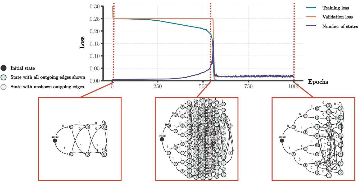
As illustrated in Figure 4, the development follows this trajectory:
- Random Initialization: The automaton is chaotic with random outputs.
- Tree Fitting (Memorization): The network expands its internal representation. It builds a “tree” where almost every unique sequence maps to a unique hidden state. At this stage, the network is memorizing the training data. It solves the task for short sequences but fails on long ones because it hasn’t learned the loop structure.
- State Merger (Generalization): This is the critical moment. Distinct branches of the tree start to collapse. States corresponding to different sequences merge into single points.
- Finite Automaton: Eventually, the automaton collapses into a finite cycle (similar to the 2-state DFA). At this exact moment, the validation loss on infinite sequences drops to zero.
The question is: Why do these states merge? Gradient descent only cares about minimizing error on the training set. A large memorization tree minimizes training error just as well as a compact DFA. What force drives the network toward the compact, generalizing solution?
The Core Method: Implicit State Merger Theory
The authors propose a theoretical framework based on local interactions between representations. They model the hidden states as particles moving in a high-dimensional space under the influence of gradient descent.
The Intuition: Continuity
The driving force is the continuity of the network’s mapping functions. In a neural network, the function mapping hidden states to outputs (\(f_y\)) is continuous. This means that if two hidden states \(h_1\) and \(h_2\) are close to each other, their predicted outputs \(y_1\) and \(y_2\) must also be close.
During training, the network updates its parameters to minimize the error between predicted outputs and target outputs. If two hidden states are somewhat close, the gradients updating the network effectively “pull” these representations based on their shared output requirements.
The Interaction Model
To formalize this, the authors model the interaction between two hidden representations, \(h_1\) and \(h_2\), corresponding to two different input sequences.
They assume the network is “expressive,” meaning it has enough parameters to approximate smooth maps freely. Instead of analyzing the complex weight updates of specific RNN architectures, they treat the hidden states and the output mappings as optimizable variables.
(Note: The schematic conceptualizes the representations \(h_1\) and \(h_2\) as adjustable points that optimize to satisfy future output requirements \(y_1 \dots y_N\).)
We look at the “local linear approximation” of the output map around the midpoint of these two representations. The output for a sequence can be approximated as:
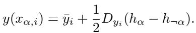
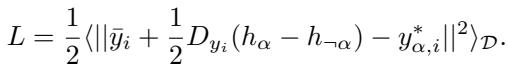
Here, \(D_{y_i}\) represents the gradient (slope) of the output function. The goal is to minimize the Mean Squared Error (MSE) loss:
The Dynamics of Attraction
By taking the gradient of this loss with respect to the hidden states and the output maps, the researchers derive a system of differential equations describing how the distance between \(h_1\) and \(h_2\) (\(||dh||^2\)) changes over time.
While the full derivation is complex, the resulting dynamics for the distance between representations can be distilled into a self-contained system. The crucial equations governing the velocity of these “particles” are:
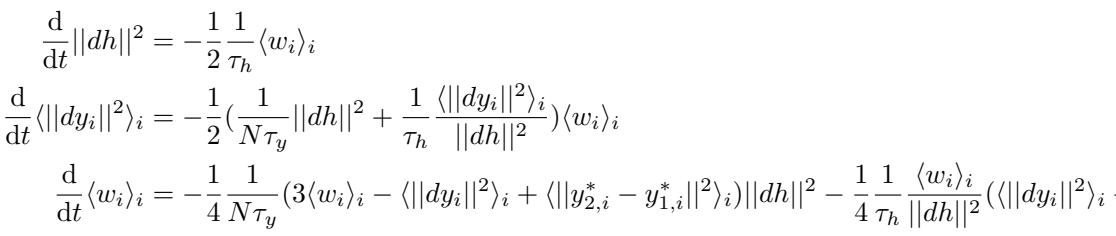
The variable \(w_i\) essentially measures the alignment between the output gradients and the target difference. The key takeaway from these dynamics is the Fixed Point Analysis. We want to know where these dynamical systems settle. Does the distance \(||dh||^2\) go to zero (merger) or stay positive (separation)?
Solving for the final representational distance yields:
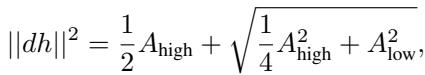
This solution depends on two critical terms, \(A_{high}\) and \(A_{low}\). The most important is \(A_{low}\), which represents the difference in target outputs:
The Merger Condition
The mathematics reveals a stark condition for two states to merge. For the distance \(||dh||^2\) to become zero (a merger), we specifically need \(A_{low} = 0\).
Looking at the definition of \(A_{low}\), this implies:
\[ \forall_i \quad y_{2,i}^* = y_{1,i}^* \]Translation: Two hidden states will merge into one if and only if they share the exact same target outputs for all possible future sequences in the training set.
If there is even a single future sequence where state \(h_1\) requires a different output than state \(h_2\), the network must keep them apart to satisfy the training loss. But if they are functionally identical regarding the future, the implicit bias of gradient descent (via continuity) creates an attractive force that collapses them together.
Furthermore, the analysis of the initial conditions shows that mergers depend on the scale of initialization. If weights are initialized to be small (scale \(G < 1\)), the attractive force is stronger for sequences where the “shared future” is long.
This explains why the network doesn’t just stay in the “Tree” phase. The tree phase separates sequences. But since many branches of the tree actually predict the same future (e.g., in Parity, any two sequences with an even number of ones are functionally equivalent), the network feels a constant pressure to merge them.
Experiments & Results
The experimental results from training standard RNNs (ReLU activations) on the Streaming Parity Task align perfectly with the theoretical predictions.
1. The “Grokking” Moment
Validation loss on long sequences remains high during the initial training phase (Tree fitting). Then, remarkably, it drops to zero almost instantaneously.
Figure 6 shows this phase transition. The fact that the drop happens for all lengths at once confirms that the network has switched from a length-dependent representation (memorization) to a length-independent one (algorithm).
2. Who Merges?
The theory predicted that only pairs of states with identical future outputs would merge. The data confirms this. Out of over 100,000 merged pairs analyzed, 100% agreed on all future outputs.
Furthermore, the theory predicted that mergers rely on sequence length. There is a threshold where the “attraction” overcomes the initial separation.
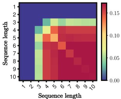
Figure 7 illustrates that short sequences (top left) rarely merge, while longer sequences (bottom right) merge frequently. This validates the theoretical finding that the merger force scales with the length of the matching future.
3. The Two-Phase Dynamics: Divergence then Merger
Why does the network fit a tree first? Why not merge immediately?
The researchers extended their interaction model to a “Fixed Expansion Point” model. This more complex model reveals that if two representations have different effective learning rates (which happens when sequence lengths differ), they will initially diverge (move apart) before the attractive force pulls them back together.
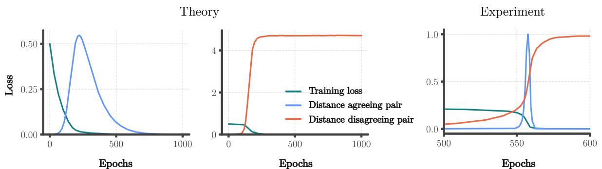
Figure 10 is a “smoking gun” for this theory.
- Theory (Left): The blue line (agreeing pair) rises (divergence) and then crashes to zero (merger). The orange line (disagreeing pair) rises and stays high.
- Experiment (Right): The RNN exhibits the exact same behavior.
This initial divergence creates the “Tree” phase. The eventual collapse creates the “Algorithm” phase.
4. Redundancy and Rich vs. Lazy Learning
The final automaton learned by the network is not always the minimal 2-state machine. It often contains redundant states—multiple states that do the same thing but didn’t manage to merge.
However, if we run a standard reduction algorithm (Hopcroft’s Algorithm) on the learned network, it collapses perfectly into the task solution.
The study also found a phase transition based on the amount of data and the weight initialization scale.
- Lazy Regime: Large initial weights or low data. The network stays in the Tree phase (memorization).
- Rich Regime: Small initial weights and sufficient data. The network enters the merging phase (algorithm learning).
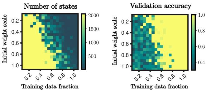
Figure 9 shows the sharp boundary between these two regimes. To get infinite generalization, you need to be in the “Rich” regime (bottom right of the heatmaps).
Transformers vs. RNNs
The paper briefly touches on Transformers. Do they exhibit the same “state merger” dynamics?
Transformers differ because they don’t have a recurrent hidden state that processes history sequentially in the same way. The authors found that Transformers do not show clear state merging in their hidden representations. However, they observed a merger-like pattern in the attention matrices.
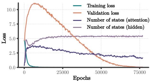
This suggests that while the mechanism of algorithm development (merging equivalent functional units) might be universal, the location of this merging depends on the architecture.
Conclusion & Implications
This research provides a concrete, mathematical explanation for how neural networks can move beyond their training data to learn true algorithms.
Key Takeaways:
- Generalization via Extrapolation: Neural networks can learn infinite algorithms from finite data, not just interpolate.
- Implicit Bias: The mechanism is the implicit bias of gradient descent combined with continuity, which pulls “functionally equivalent” representations together.
- Phase Transition: Learning happens in two distinct stages: memorizing the data (Tree) followed by compressing the logic (State Merger).
- Representational Dynamics: We can model these complex networks as systems of interacting particles to predict when and how they will learn.
This work bridges the gap between the black-box nature of Deep Learning and the structured logic of Computer Science. For neuroscience, it suggests that “redundant” neural representations might be a natural artifact of learning dynamics. For AI safety, it highlights the specific conditions (initialization, data volume) required to ensure a model learns the robust algorithm rather than a brittle heuristic.
By understanding these dynamics, we move one step closer to engineering networks that don’t just memorize, but truly understand the rules governing their data.