Introduction: The Mapmaker’s Dilemma in Biology

Imagine you are trying to navigate across a globe, but you only have a flat paper map. You draw a straight line with a ruler from New York to London. On your map, it looks like the shortest path. But if you were to fly that route in reality, you would realize that because the Earth is curved, your “straight line” on the map is actually a longer, inefficient curve on the globe. The shortest path on the sphere (a geodesic) looks curved on your flat map.

This geometric mismatch is the exact problem researchers face when analyzing single-cell RNA sequencing (scRNA-seq) data using Deep Learning.

In computational biology, we use Variational Autoencoders (VAEs) to compress the massive complexity of thousands of genes into a low-dimensional “latent space”—a simplified map of cellular identity. We love this latent space because it allows us to perform linear interpolation. We take a stem cell (point A) and a mature cell (point B), draw a straight line between them in the latent space, and assume that the points along that line represent the biological steps the cell takes to mature.

But here is the catch: Standard VAEs do not guarantee that the latent space is flat.

Just like the Mercator projection distorts the size of continents, a standard VAE distorts biological distances. A straight line in the latent space might correspond to a wild, biologically impossible trajectory in the actual gene expression space.

Enter FlatVI, a new framework introduced by Palma, Rybakov, et al., which forces the VAE to learn a latent space that is actually flat (Euclidean). By enforcing geometry during training, FlatVI ensures that straight lines in the latent map correspond to meaningful, geodesic paths in the complex world of cell biology.

In this post, we will tear down the mathematics of FlatVI, explore how it utilizes Riemannian geometry and the Fisher Information Metric, and see why “flattening” the curve is crucial for understanding how cells develop.

Background: The Shape of Data

To understand FlatVI, we first need to set the stage with the tools of the trade: VAEs, Riemannian Geometry, and the specific nature of single-cell data.

Single-Cell RNA-seq and VAEs

Single-cell RNA sequencing gives us a snapshot of the activity of thousands of genes inside a single cell. Because this data is high-dimensional (often 20,000+ dimensions per cell) and noisy, we use VAEs to learn a compressed representation.

A VAE consists of two parts:

1. The Encoder: Compresses the high-dimensional gene counts (\(x\)) into a low-dimensional latent vector (\(z\)).
2. The Decoder: Reconstructs the original data from the latent vector.

Mathematically, the decoder defines a likelihood model. For single-cell data, we don’t just output numbers; we output the parameters of a probability distribution.

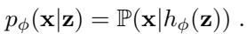
Here, \(h_{\phi}(z)\) is the decoder neural network. It maps a latent point \(z\) to the parameters of a distribution that generates the data \(x\).

The Geometric Disconnect

The core issue is how we measure distance. In the latent space \(\mathcal{Z}\), we usually assume the geometry is Euclidean. This means the distance between two points is just the standard straight-line distance (like using a ruler).

However, the data usually lies on a curved “manifold” (a shape) embedded in the high-dimensional space. The decoder \(h\) maps our simple latent space onto this complex manifold.

If we don’t restrict the decoder, it can twist and stretch the latent space however it wants. A small step in one part of the latent space might result in a huge jump in gene expression, while a large step in another part might barely change the cell’s state. This varying “speed” of change means the latent space has a non-Euclidean geometry.

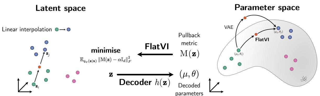
As shown in Figure 1, standard VAEs (top path) allow straight lines in latent space to map to curves that stray off the optimal path on the manifold. FlatVI (bottom path) forces the latent straight lines to map directly to the shortest paths (geodesics) on the manifold.

The Core Method: Enforcing Flatness

How do we force a neural network to respect Euclidean geometry? We have to measure the curvature and penalize it during training. This involves a concept called the Pullback Metric.

The Pullback Metric

Imagine you are walking on a landscape (the manifold). You have a map (the latent space) in your pocket. The metric tensor \(M(z)\) tells you how to translate a step on your map into a real physical distance on the landscape.

If the map is perfectly accurate (flat and undistorted), the metric tensor is just the Identity matrix (\(I\)). Every step on the map equals one constant step in reality. If the map is distorted, \(M(z)\) changes depending on where you are.

In a VAE, we can calculate this metric by looking at how the decoder changes. Specifically, we use the Jacobian \(\mathbb{J}_h(z)\), which measures the sensitivity of the output relative to the input.

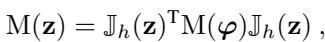
This equation states that the metric in the latent space \(M(z)\) is the metric of the data space \(M(\phi)\) “pulled back” through the decoder.

The Statistical Manifold and Fisher Information

Here is where it gets interesting. Since the VAE outputs probability distributions, the “data space” isn’t just a physical surface; it is a Statistical Manifold. The points on this manifold are probability distributions.

The natural way to measure distance between distributions is the Fisher Information Metric (FIM).

The FIM measures how distinguishable two probability distributions are. If changing the parameters slightly makes the distribution look very different, the FIM is high (large distance). If the distribution looks basically the same, the FIM is low.

By plugging the FIM into our pullback equation, we get a metric \(M(z)\) that tells us how fast the probability distribution of the data changes as we move through the latent space.

The Flattening Loss

The goal of FlatVI is simple: we want the latent space metric \(M(z)\) to look like a scaled Identity matrix everywhere. If \(M(z) \approx \alpha \mathbb{I}\), it means the curvature is zero—the space is flat.

The authors propose a regularization term, the Flattening Loss:

This loss function calculates the difference (Frobenius norm) between the actual calculated metric \(M(z)\) and a target flat metric \(\alpha \mathbb{I}_d\).

We add this term to the standard VAE loss function (the ELBO). This creates a tradeoff: the model must reconstruct the data accurately (ELBO) while keeping the latent space flat (Flattening Loss).

\(\lambda\) is a hyperparameter that controls how strictly we enforce the flatness.

Tailoring for Single-Cell: The Negative Binomial Case

One of the major contributions of this paper is deriving the specific metric for Negative Binomial (NB) distributions, which are the standard noise model for scRNA-seq count data.

Most previous geometric autoencoders assumed Gaussian data (continuous), which fits poor on discrete gene counts. The authors explicitly model the sparsity and overdispersion of biological data.

The Negative Binomial distribution is defined as:

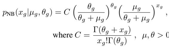
Here, \(\mu_g\) is the mean expression of a gene, and \(\theta_g\) is the inverse dispersion (how spread out the counts are).

The authors derived the exact pullback metric for this specific likelihood. This allows FlatVI to be mathematically rigorous specifically for sequencing data:

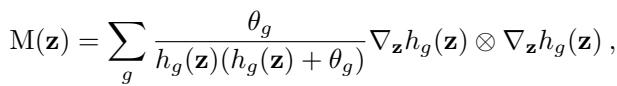
This equation might look intimidating, but it is the engine of the method. It tells the network exactly how to adjust the weights to ensure that changes in the latent variable \(z\) result in consistent, “flat” changes in the Negative Binomial output distributions.

Experiments and Results

Does forcing this geometry actually work? The authors put FlatVI to the test on simulated data and real-world biological datasets.

Simulation: Verifying the Geometry

First, they created a synthetic dataset where the ground truth geometry is known. They compared a standard Negative Binomial VAE (NB-VAE) against FlatVI with increasing regularization strength (\(\lambda\)).

They measured two key properties of the latent space:

1. Variance of the Riemannian Metric (VoR): Ideally 0. A measure of how much the “ruler” changes size as you move around.
2. Condition Number (CN): Ideally 1. A measure of how much the space is stretched in different directions.

Figure 2 visualizes these metrics.

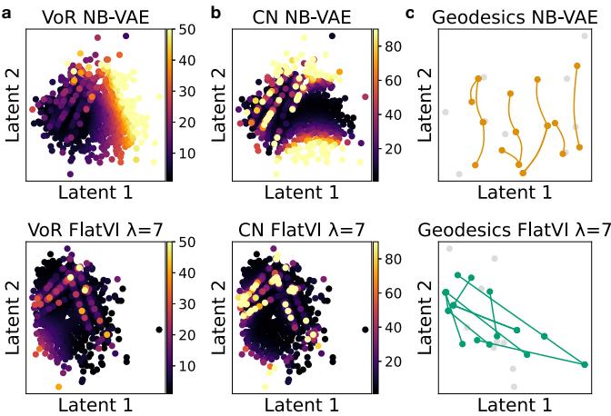
In the standard VAE (top row), you see “hot spots” (yellow/red) where the metric is highly distorted. In FlatVI (bottom row), the space is much cooler (purple/blue), indicating a uniform, flat geometry.

Furthermore, Figure 2(c) shows the geodesic paths. In the standard VAE, the shortest path between two points is a curve. In FlatVI, the shortest path is a straight line—exactly what we want for linear interpolation.

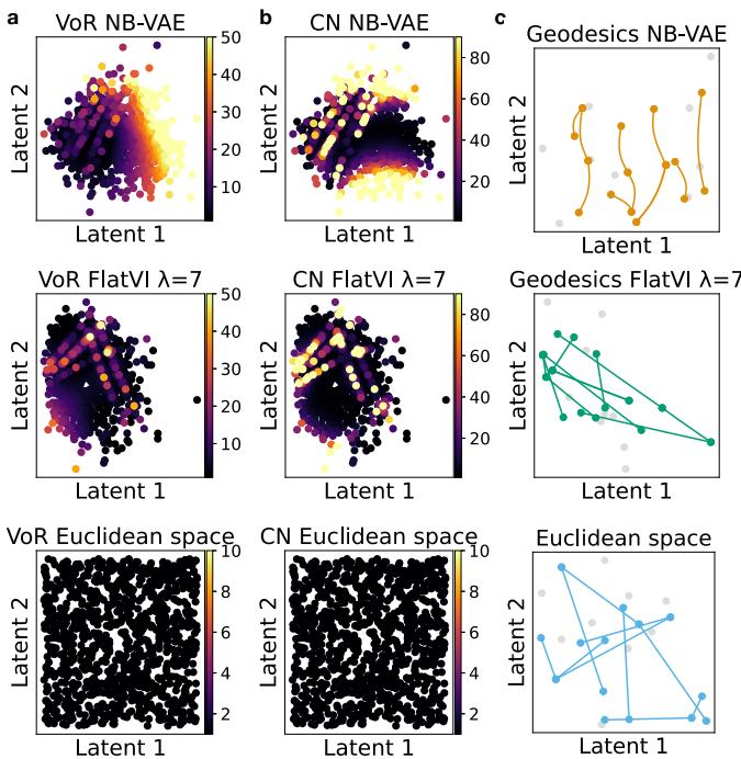
For comparison, Figure 7 below shows what a perfectly Euclidean space looks like (bottom row). FlatVI (middle row) approximates this ideal structure much better than the standard VAE (top row).

Trajectory Inference: Predicting Cell Development

The real test is biological data. Cells differentiate over time (e.g., from a stem cell to a heart cell). This is a continuous process.

The authors used Optimal Transport (OT) to model these trajectories. OT is a mathematical framework for moving mass from one distribution to another efficiently. Specifically, they used OT-CFM (Conditional Flow Matching), a method that assumes straight-line paths between time points.

Since OT-CFM assumes straight lines, it works best if the underlying representation supports straight lines.

Figure 12 shows the results on an Embryoid Body (EB) dataset. The goal was to predict the state of cells at an intermediate time point that was held out during training.

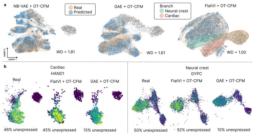
FlatVI (right panel in Figure 12a) achieves a much tighter overlap between the predicted cells and the real cells compared to the baselines (GAE and NB-VAE). This proves that the “flat” map created by FlatVI is a more accurate representation of the biological process.

Biological Consistency: Vector Fields

Another way to validate the model is to look at RNA velocity and vector fields. We can infer the direction a cell is moving in the latent space. If the latent space is well-structured, these vectors should flow smoothly from stem cells to terminal cell types.

Figure 11 compares the vector fields on Pancreas data.

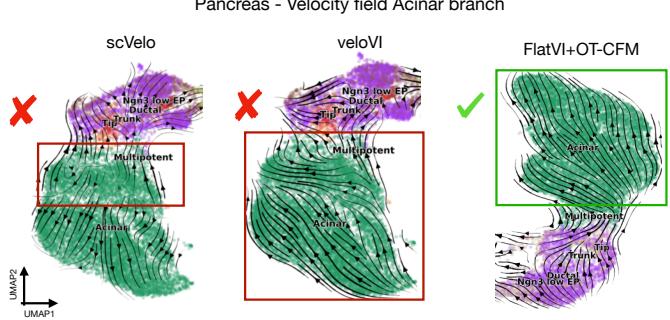
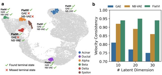
FlatVI successfully captures the branching lineages. Even more impressively, when using CellRank (a tool to find terminal states), FlatVI identified all 6 known terminal cell types in the dataset. Standard methods like NB-VAE and GAE missed some of them.

Linear Interpolation: The Ultimate Test

Finally, the authors returned to the original motivation: Manifold Interpolation. Can we just draw a straight line between two cells and generate a biologically realistic movie of development?

They compared FlatVI against GAGA (a geometry-aware geometric autoencoder). They took a multipotent cell and a mature cell, interpolated linearly in latent space, and decoded the gene expression along the path.

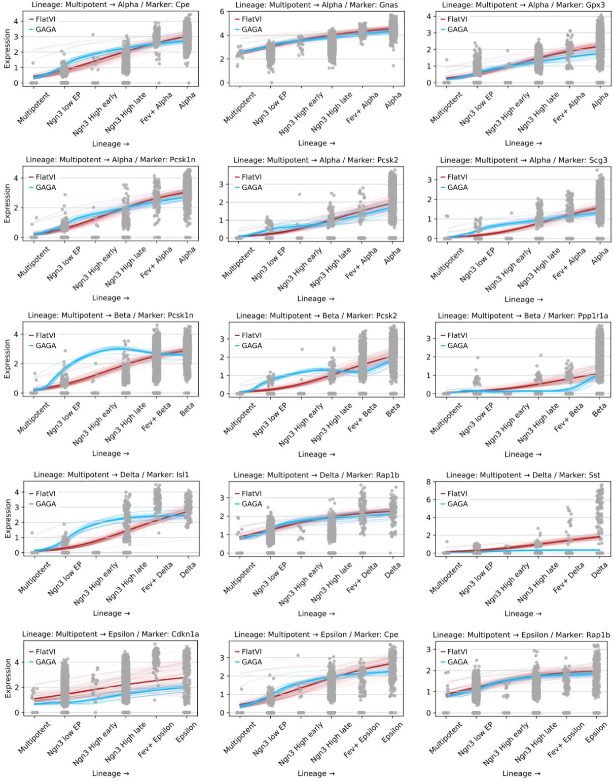
As shown in Figure 13 (and Figure 5 in the paper), FlatVI produces smooth, monotonic trends for marker genes (like Cpe and Nnat). This confirms that a straight walk in the FlatVI latent space corresponds to a smooth biological progression.

Crucially, because FlatVI enables linear interpolation, it is computationally much faster than methods that require solving differential equations to find geodesics.

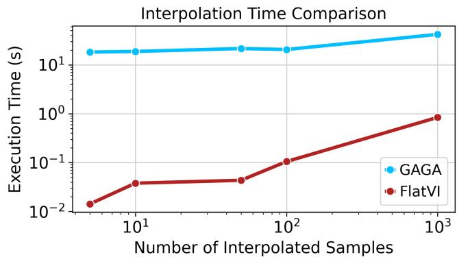
Note on Figure 14: While GAGA (blue) appears faster in raw seconds for small samples in this specific plot, the key advantage of FlatVI is the simplicity of the operation—simple linear algebra vs. solving neural ODEs. FlatVI scales gracefully and allows for instant path generation once the model is trained.

Conclusion and Implications

FlatVI represents a significant step forward in ensuring that our machine learning models respect the geometry of the data they represent. By regularizing the latent space to be locally Euclidean, the authors achieved:

1. Theoretical Soundness: Aligning the latent metric with the Fisher Information Metric of the Negative Binomial decoder.
2. Better Dynamics: Improved performance in Optimal Transport trajectory inference.
3. Interpretability: Enabling simple linear interpolations to reveal complex biological pathways.

For students and researchers, this paper underscores an important lesson: Architecture isn’t everything; Geometry matters. You can’t just shove data into a standard VAE and assume the latent space makes sense. By explicitly enforcing geometric constraints—“flattening the map”—we can build tools that are not only mathematically rigorous but also biologically faithful.

Whether you are modeling stem cells, cancer evolution, or drug responses, knowing that your “straight line” is actually the shortest path makes all the difference in navigating the complex landscape of biology.

References and Further Reading:

• This post is based on the paper “Enforcing Latent Euclidean Geometry in Single-Cell VAEs for Manifold Interpolation” by Palma, Rybakov, et al. (2025).
• Figures used in this post are extracted directly from the paper’s image deck.