Introduction: The Noise in the Air

In the modern world, the air around us is saturated with invisible data. From cellular networks to military radar, electromagnetic signals are constantly crisscrossing the atmosphere. Managing this chaotic spectrum requires Automatic Modulation Classification (AMC). This technology acts as a digital gatekeeper, identifying the type of modulation (the method used to encode data onto a radio wave) of a detected signal. Whether it is for dynamic spectrum allocation or surveillance, the system must know: Is this a 64QAM signal? Or perhaps QPSK?

Deep learning has revolutionized AMC, replacing rigid feature engineering with neural networks that learn to recognize signal patterns directly. However, a persistent problem remains. When signal-to-noise ratios (SNR) drop, or when modulation schemes look incredibly similar (like distinguishing between QPSK and 8PSK), deep learning models tend to hesitate. They suffer from prediction ambiguity.

Instead of confidently saying, “This is Class A,” the model essentially shrugs, assigning a 45% probability to Class A and a 42% probability to Class B. This ambiguity kills reliability.

In this post, we are diving deep into a recent paper, “Robust Automatic Modulation Classification with Fuzzy Regularization,” which proposes a mathematical solution to this “laziness” in neural networks. The researchers introduce Fuzzy Regularization (FR), a technique that forces models to stop hedging their bets and learn sharper, more robust decision boundaries.

The Core Problem: Prediction Ambiguity

To understand the solution, we first need to understand why deep learning models fail here. In ideal conditions, a classifier outputs a “one-hot” style probability: 99% for the correct class and near 0% for the rest.

However, in the domain of signal processing, modulation types often differ only by subtle coding bits, while their physical waveforms (In-Phase and Quadrature components) look nearly identical under noise.

The authors of the paper identified that this leads to “soft” distributions in the output layer (Softmax).

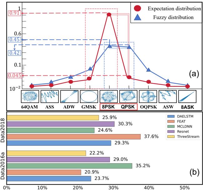
As shown in Figure 1(a) above, the blue line represents a typical ambiguous prediction. The top two probabilities are nearly indistinguishable (e.g., 0.45 vs 0.42). The red line represents the ideal, sharp prediction we want.

In Figure 1(b), the authors show that this isn’t a fluke. Across different architectures (ResNet, LSTM, etc.) and datasets, approximately 25% of samples suffer from this ambiguity. The model hasn’t learned the distinguishing features; it has simply learned that it’s safer to be vague than to be wrong.

Why Does the Model Get Lazy? A Probabilistic Perspective

Why doesn’t standard training (using Cross-Entropy Loss) fix this? The researchers modeled this phenomenon mathematically to find the root cause.

Let’s imagine a binary classification task with a batch of samples \(k\). If the model is confused, the highest predicted probability for a class tends to stabilize around a constant value \(u\).

The standard Cross-Entropy loss for a batch is calculated as:

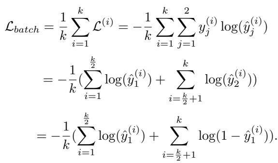
If we assume the model is struggling to differentiate two classes, the classification accuracy \(\alpha\) essentially becomes a coin toss (0.5). By modeling the expected loss \(E(\mathcal{L}_{batch})\) based on the probability of misclassification, the researchers derived the following relationship:

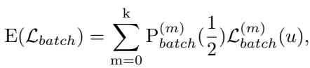
Through further derivation, they arrived at a critical insight regarding the expected loss behavior relative to the prediction probability \(u\):

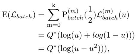
The takeaway: The mathematics reveal that when the model cannot find distinct features, the expected loss reaches a minimum when \(u = 0.5\). In plain English, the loss function effectively rewards the model for being ambiguous when the data is hard. The model settles into a “lazy” state, smoothing out its predictions to control the growth of the loss rather than trying to solve the hard problem of distinguishing similar classes.

The Solution: Fuzzy Regularization (FR)

To break the model out of this lazy local minimum, we need to penalize ambiguity. We need a Regularization term—an extra component added to the loss function that says, “I don’t just care that you classify correctly; I care how certain you are.”

Attempt 1: Entropy and Variance (and why they fail)

The most common ways to measure “disorder” or ambiguity are Entropy and Variance (L2 Norm).

• Entropy: High entropy means high disorder (ambiguity).
• L2 Norm (Variance): Low variance means the probabilities are spread out flatly (ambiguity).

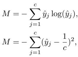
The researchers considered defining a penalty \(M\) based on these concepts:

However, simply adding these to the loss function caused training instability. The reason lies in the gradients.

Look at Figure 7(a) above. This graph shows the gradient (slope) of the entropy function. The problem is that even when the prediction ambiguity is low (meaning the model is becoming confident), the entropy function still returns a relatively large gradient update. This causes the model parameters to oscillate wildly just as they are getting close to the optimal solution, preventing convergence.

Attempt 2: The Adaptive Gradient Mechanism

The researchers realized they needed a “smart” penalty.

1. High Ambiguity: Return a large loss and a large gradient to force the model to change.
2. Low Ambiguity: Return a small gradient to allow the model to fine-tune stably.

They designed a regularization curve that behaves like the function \(y = -\log(|x| - 0.5)\).

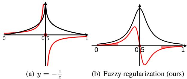
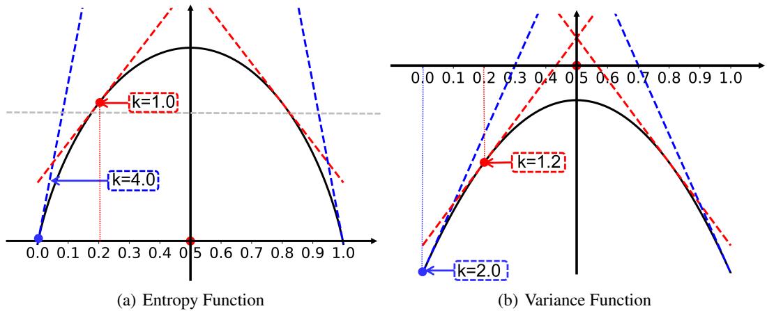
In Figure 2(b), you can see the proposed Fuzzy Regularization (FR) curve. It creates a “hump” where ambiguity is highest. As the model pushes predictions away from the ambiguous center (0.5) toward 0 or 1, the gradient (red line) naturally decreases, stabilizing the training.

The Mathematical Formulation of FR

To implement this, the authors utilized a Log-Normal Distribution function to construct the final regularization term. This combines the ambiguity of individual samples with the statistics of the whole batch.

First, they defined a loss based on the L2 norm for a single sample, normalized to focus purely on the distribution shape:

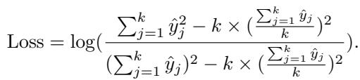
Then, they integrated this into the final Fuzzy Regularization function \(F(\hat{y})\):

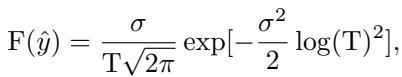
Subject to the following parameters, where \(T\) represents the variance statistics of the top-\(k\) predicted classes:

This looks complex, but the mechanism is elegant: It dynamically re-weights samples. If a sample is ambiguous, the FR term spikes, dominating the loss and forcing the network to focus on that “hard” sample. As the sample becomes clear, the FR term vanishes, letting the standard Cross-Entropy loss handle the fine details.

Experimental Results

Does this math hold up in the real world? The researchers tested FR-AMC on three benchmark datasets: RadioML 2016.10a, 2016.10b, and 2018.01A. They applied the FR module to five different state-of-the-art models (including ResNet, LSTM, and Transformers) to prove it works regardless of the architecture.

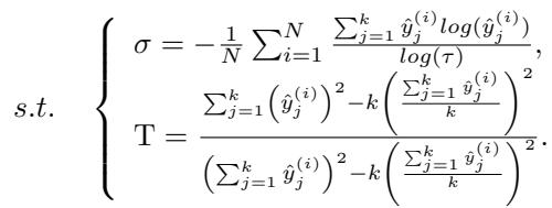
1. Generalization Comparison

The results were consistent. Adding Fuzzy Regularization improved performance across the board.

As seen in Table 2, every single model (DAELSTM, FEAT, MCLDNN, etc.) saw an improvement in Accuracy (ACC) and F1-Score when “FR” was added.

• Key Insight: The improvement was most drastic on “harder” datasets (Data2016a) where prediction ambiguity is more common. On Data2016b, where baseline models already score >90%, the gain was smaller but still positive. This confirms FR specifically targets the “hard” cases.

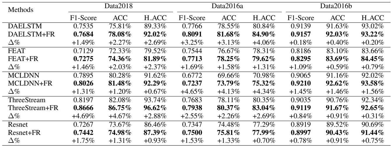
2. Robustness Against Noise

The true test of a radio system is noise. The researchers generated “Noisy” versions of the datasets with varying noise factors (20%, 40%, 60%).

Table 3 shows that as noise increases, the gap between the baseline and the FR-enhanced models widens. For example, on Noise2016b with 60% noise, the MCLDNN model’s accuracy jumped from 59.02% to 74.31% just by adding FR. This suggests that by forcing the model to be less ambiguous during training, it learns feature representations that are much more resilient to interference.

3. Visualizing the Decision Boundary

Numbers are great, but seeing the data clusters is better. The researchers used t-SNE to visualize how the model separates two very similar modulation types: 8PSK (Red) and QPSK (Blue).

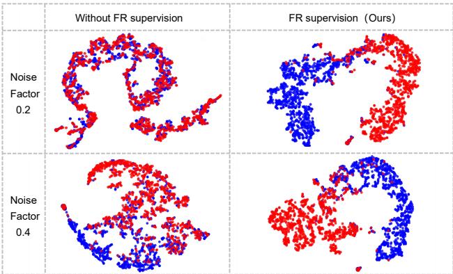
In Figure 3, the top row (No FR) shows the clusters “smearing” into each other, especially as noise increases. The bottom row (With FR) shows tighter, more distinct clusters. The FR penalty has effectively forced the model to maximize the margin between these confusable classes.

4. Training Speed and Stability

Finally, did this extra complexity slow down training? Surprisingly, no.

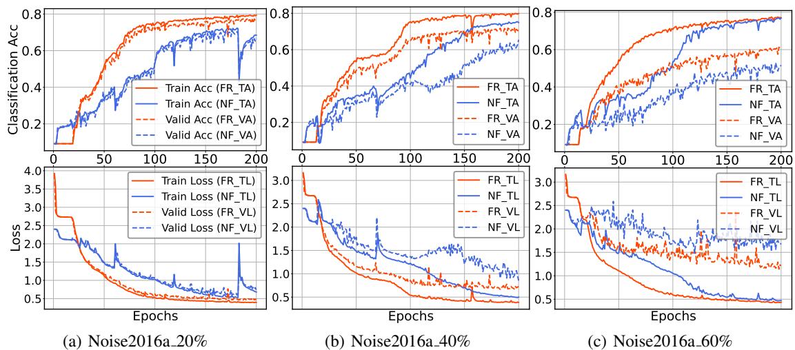
Figure 4 compares the training curves. The Red line (FR) converges faster and smoother than the Blue line (No FR).

• Curriculum Learning Effect: By sharpening the easy predictions early, the model can stop worrying about them and devote its gradient updates to the hard, ambiguous samples. This acts like an automatic “curriculum,” speeding up the learning process.

Conclusion

The “Robust Automatic Modulation Classification with Fuzzy Regularization” paper highlights a subtle but critical flaw in how we train deep learning models for signal processing: the tendency to accept ambiguity.

By mathematically modeling this laziness and designing a Fuzzy Regularization term with an adaptive gradient, the researchers provided a plug-and-play module that:

1. Penalizes Uncertainty: Forces the model to make a choice.
2. Stabilizes Training: Reduces gradients as confidence grows.
3. Boosts Robustness: dramatically improves performance in high-noise environments.

For students and practitioners in AMC, this is a valuable lesson. It is not always about building a bigger, deeper neural network. Sometimes, the key to better performance lies in the loss function—changing how the model learns, not just what it learns. By refusing to accept “maybe” as an answer, FR pushes models to understand the true nature of the signals they analyze.