Introduction

In the era of deep learning, data is the new oil. But raw data is useless without accurate labels. While we would love to have domain experts annotate every single image or document, that is often prohibitively expensive and slow. Enter crowdsourcing: a method where tasks are distributed to a large pool of non-expert workers (like on Amazon Mechanical Turk).

Crowdsourcing is cost-effective, but it introduces two major headaches:

1. Noise: Crowd workers make mistakes.
2. Sparsity: Workers usually answer only a tiny fraction of the available questions.

To handle noise, we typically use Label Aggregation (voting mechanisms) to infer the true label from multiple workers. However, aggregation algorithms struggle when the data is sparse. If a specific image was only labeled by one or two unreliable workers, majority voting fails.

This brings us to Label Completion—a preprocessing step where we try to intelligently “fill in the blanks” of the label matrix before we aggregate the votes.

In this post, we are diving into a 2025 paper titled “TLLC: Transfer Learning-based Label Completion for Crowdsourcing.” The authors propose a clever solution to a specific problem in label completion: How do you model a worker’s behavior when they have hardly annotated anything? Their answer lies in Transfer Learning.

The Problem: Insufficient Worker Modeling

Current state-of-the-art methods try to predict missing labels by modeling the “personality” or reliability of each worker. If we know Worker A is great at identifying dogs but bad at cats, we can weigh their votes accordingly or predict how they would have voted.

However, there is a catch-22. To build a good model of Worker A, we need plenty of data from them. But in real-world scenarios, workers often annotate very few instances. This leads to insufficient worker modeling. The model fails to capture the worker’s characteristics, leading to bad predictions for the missing labels.

The Solution: TLLC

The researchers propose Transfer Learning-based Label Completion (TLLC). The core idea is simple yet powerful: instead of training a model for each worker from scratch (which fails due to lack of data), we first train a “general” model on the high-confidence data from the entire crowd (the Source Domain). Then, we transfer this knowledgeable model to the individual worker (the Target Domain) and fine-tune it.

This allows the model to learn general features from the group, while still adapting to the specific quirks of the individual worker.

The TLLC Framework

Let’s look at the overall workflow of the TLLC method.

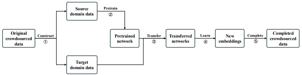
As shown in Figure 1, the process breaks down into five distinct steps:

1. Construct source and target domains.
2. Pretrain a Siamese network on the source domain.
3. Transfer the network to specific workers.
4. Learn embeddings.
5. Complete the missing labels.

Let’s break these down in detail.

Step 1: Constructing the Source and Target Domains

Before any training happens, we need to organize our data. The Target Domain is easy—it’s just the data annotated by a specific worker.

The Source Domain is trickier. We want a large dataset of “high-quality” examples to pre-train our network. But we don’t have ground truth labels; we only have noisy crowd votes. The authors use a technique inspired by confident learning to filter the data.

First, they calculate the initial aggregated label \(\hat{y}_i\) for an instance (likely the majority vote) and the probability (confidence) of that label.

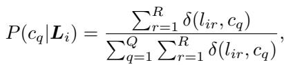
Next, they calculate the average confidence threshold \(\mu\) for each class. This sets a bar for quality: if an image is labeled “cat,” is the confidence higher than the average confidence for all “cat” images?

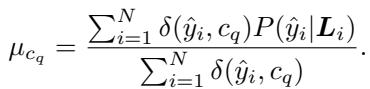
Finally, they construct the Source Domain (\(X_S\)) by keeping only the instances where the confidence score exceeds the average threshold for that class.

By doing this, the researchers effectively create a “Silver Standard” dataset—it’s not perfect ground truth, but it’s the highest-confidence data available from the crowd.

Step 2 & 3: Worker Modeling via Siamese Networks

Now that we have data, how do we model the workers? The authors choose a Siamese Network architecture.

Siamese networks are designed to measure similarity. They take two inputs and output a distance metric—if two images have the same label, the network learns to put them close together in the embedding space. If they have different labels, it pushes them apart.

The Transfer Learning Twist:

1. Pre-training: The network is first trained on the high-quality Source Domain. Since this dataset is large, the network learns robust feature representations (embeddings) of the data.
2. Transfer & Fine-tuning: The weights of this pre-trained network are then copied to a specific worker’s network. This network is then fine-tuned using only the few instances that specific worker annotated (the Target Domain).

This approach solves the sparsity problem. Even if a worker only labeled 5 items, their specific model starts with a rich understanding of the data thanks to the pre-training.

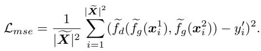
The training uses a Mean Squared Error (MSE) loss function to minimize the difference between the predicted distance of two items and their actual relationship (0 if same class, 1 if different).

Step 4 & 5: Label Completion

Once the worker-specific network is trained, it can generate a new embedding vector (denoted as \(z\)) for any instance.

To predict a missing label for a worker:

1. The authors calculate the centroid (average position) of all instances the worker labeled as Class A, Class B, etc.
2. They define a “safe radius” (average distance) around these centroids.
3. For an unlabeled instance, they map it into this space.

If the unlabeled instance falls close enough to the centroid of a specific class (closer than the average distance calculated), the algorithm assigns that label to the instance.

The formal condition for completion is:

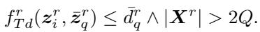
Here, the distance between the instance \(z_i\) and the class centroid \(\bar{z}_q\) must be less than the threshold \(\bar{d}_q\).

Experiments and Results

To prove this method works, the authors tested TLLC against state-of-the-art baselines, including a method called WSLC (Worker Similarity-based Label Completion). They used real-world datasets: Income (binary classification), Leaves (6 classes), and Music_genre (10 classes).

Does it improve accuracy?

The primary metric is Aggregation Accuracy—after filling in the missing labels using TLLC, how accurately can we determine the true label?

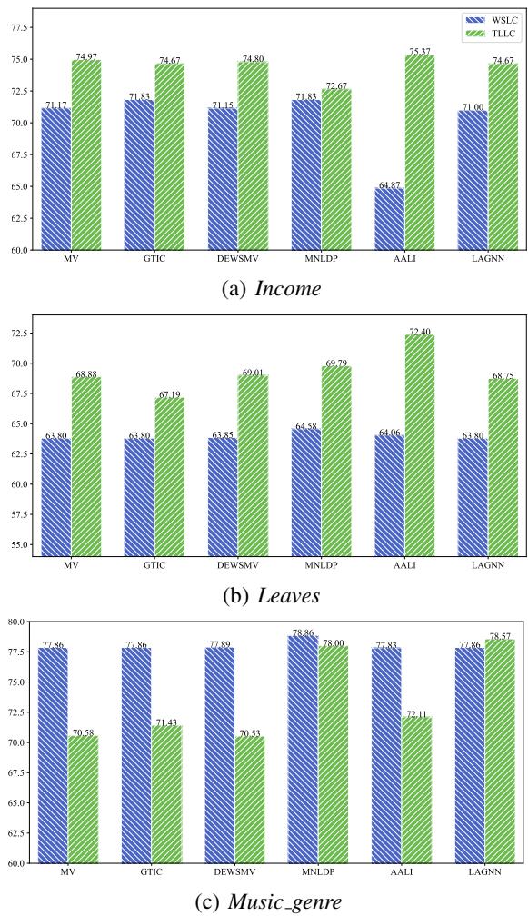
As shown in Figure 2, TLLC (the green/striped bars) consistently outperforms or matches the baseline WSLC (blue bars).

• Income & Leaves: TLLC shows significant improvements across almost all aggregation methods (MV, GTIC, etc.).
• Music_genre: The performance is competitive, though the gap is smaller.

Why does Transfer Learning matter?

The most compelling proof in the paper is the visualization of the embeddings. The authors took a worker who had annotated very few instances and visualized how the network “sees” the data with and without transfer learning.

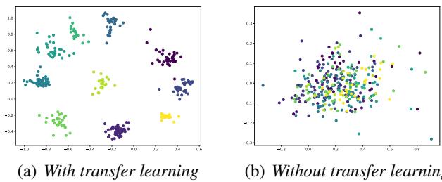
• Right (Without Transfer Learning): The points are a jumbled mess. The model hasn’t seen enough data to separate the classes.
• Left (With Transfer Learning): The classes (colors) are distinct and clustered. Even though this specific worker provided little data, the pre-training allowed the model to understand the structure of the dataset.

Preserving Worker Characteristics

A risk in label completion is “homogenization”—making every worker look like the average. However, valid crowdsourcing relies on diversity.

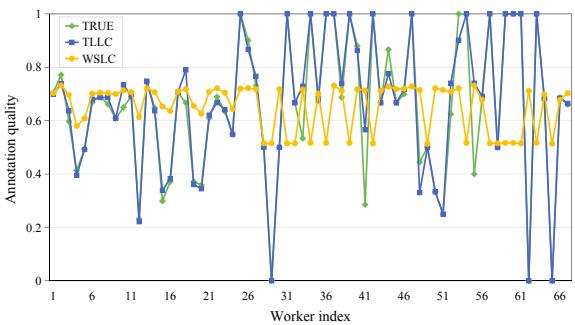
Figure 6 shows the annotation quality of workers. The orange line (WSLC) shows that the baseline method tends to flatten the curve, making bad workers look better and good workers look worse—it’s averaging them out. The blue line (TLLC) tracks closer to the green line (True quality), meaning TLLC respects the unique capability level of each worker while still filling in their missing data.

Conclusion

The TLLC method addresses a critical gap in crowdsourcing: the inability to model workers who simply haven’t done enough work yet. By treating the collective high-confidence data as a Source Domain and the individual worker as a Target Domain, the researchers successfully applied Transfer Learning to stabilize the process.

Key Takeaways:

1. Don’t start from scratch: In sparse data environments, leverage the global dataset to pre-train models for individuals.
2. Filter first: Using confident learning to create a clean Source Domain is essential for effective pre-training.
3. Embeddings work: Siamese networks allow us to complete labels based on geometric similarity, which is often more robust than simple probability.

This research paves the way for more efficient crowdsourcing platforms that can get accurate results with fewer annotations, saving both time and money.