Unlocking Causal Secrets: How to Efficiently List Hidden Variable Graphs

In the world of Artificial Intelligence and Causal Inference, we often deal with incomplete pictures. We observe data—like symptoms in a patient or economic indicators in a country—but we rarely see the full machinery driving these observations. There are almost always “latent variables,” hidden factors that influence what we see but remain unrecorded.

When we try to map out causal relationships in the presence of these hidden factors, we don’t get a single, clear map. Instead, we get a “class” of possible maps. Navigating this class to find every specific, valid causal explanation is a massive computational headache.

Today, we are diving into a recent research paper that solves a critical bottleneck in this field. We will explore MAGLIST-POLY, an algorithm that can list all possible causal graphs (specifically Maximal Ancestral Graphs, or MAGs) with polynomial delay. This is a significant leap forward from previous exponential-time methods, allowing researchers to explore causal possibilities much faster.

The Landscape of Causal Graphs

To understand the solution, we first need to understand the problem. Let’s break down the hierarchy of causal graphs.

From DAGs to PAGs

In an ideal world, if we measured every relevant variable, we could represent causality with a Directed Acyclic Graph (DAG). In a DAG, an arrow from \(A \rightarrow B\) means \(A\) causes \(B\).

However, in the real world, we have latent confounders (hidden common causes) and selection bias (unrecorded factors influencing data collection). When these exist, a simple DAG of observed variables isn’t enough. We use a Maximal Ancestral Graph (MAG) to represent causal relations among the variables we can see, while implicitly accounting for the ones we can’t.

Here is the catch: multiple different MAGs can generate the exact same statistical patterns in the data. This set of statistically indistinguishable MAGs is called a Markov Equivalence Class (MEC).

Since we can’t tell these MAGs apart using only observational data, we summarize the entire class into a single object called a Partial Ancestral Graph (PAG).

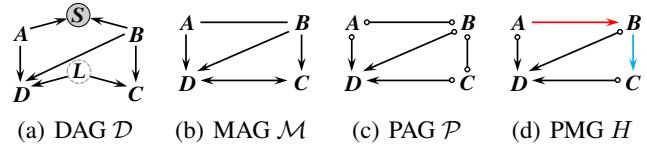
Figure 1 illustrates this hierarchy:

• (a) DAG: The ground truth with hidden variables \(L\) and \(S\).
• (b) MAG: The representation of causal relations among observed variables (\(A, B, C, D\)).
• (c) PAG: What we actually learn from data. Notice the circles (\(\circ\)). These represent uncertainty. An edge \(A \circ\!\to B\) means “we know there is a connection, and \(B\) is not an ancestor of \(A\), but we don’t know if \(A\) causes \(B\) or if there is a hidden confounder.”

The Problem: Listing the Possibilities

The PAG (Figure 1c) is useful, but it is vague. For many downstream tasks—like estimating the causal effect of a drug or designing the most efficient experiment to distinguish between hypotheses—we need to look at the specific underlying MAGs.

We need a way to take a PAG and say, “Here is the list of every specific MAG that could possibly exist within this summary.” This process is called MAG Listing.

The Computational Bottleneck

Listing MAGs is much harder than listing DAGs because MAGs have more edge types (directed \(\to\), bi-directed \(\leftrightarrow\), and undirected \(-\)).

The previous state-of-the-art method, known as MAGLIST, used a recursive approach. It would pick a node (variable) and try to resolve all the uncertain edges connected to it simultaneously. While effective, this approach has a major flaw: Exponential Delay.

Delay refers to the time it takes the algorithm to output the next valid graph after finding the previous one. Because MAGLIST tries to enumerate every combination of edges around a node at once (a “local structure”), the complexity grows exponentially with the number of neighbors (\(2^d\)).

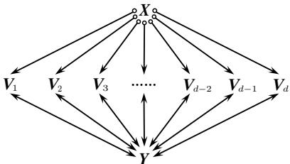
As shown in Figure 7, if a node \(X\) connects to many other nodes (\(V_1\) to \(V_d\)), trying to resolve all those circles at once creates a massive fan-out of possibilities, bogging down the system.

The Solution: MAGLIST-POLY

The researchers behind this paper propose a refined approach: MAGLIST-POLY. The goal is to achieve polynomial delay, meaning the time to find the next graph scales manageably with the size of the graph, not exponentially.

The Strategy: Singleton Background Knowledge

The core insight is simple but powerful. Instead of trying to guess the orientation of all edges connected to a node simultaneously, why not guess them one by one?

This concept relies on Background Knowledge (BK). BK is external information we assume to be true (like “we know A causes B”).

• Local BK: Guessing all edges around a node (used by the old MAGLIST).
• Singleton BK: Guessing the orientation of just one specific edge or circle.

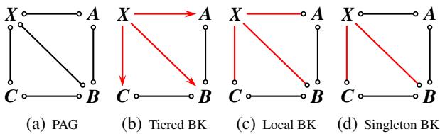
Figure 3 visualizes this difference.

• (c) Local BK: We define relationships between \(X\) and all its neighbors (\(A, B, C\)).
• (d) Singleton BK: We define the relationship only between \(X\) and one neighbor (\(B\)).

By introducing Singleton BK, the algorithm avoids the exponential explosion. It makes a small choice, propagates the implications of that choice, and then moves on.

The Challenge: “Local Completeness”

You might ask, “If doing it one-by-one is faster, why didn’t we always do that?”

The danger of making small, incremental choices is that you might paint yourself into a corner. You might orient an edge \(A \to B\) in a way that looks fine locally, but implies a contradiction five steps down the road that you can’t see yet. If you don’t realize this immediately, you waste time exploring invalid branches of the search tree.

To make Singleton BK work, we need Orientation Rules. These are logical rules that say, “If \(A \to B\) and \(B \to C\), you must orient the edge between \(A\) and \(C\) as…”

For the polynomial delay guarantee to hold, the orientation rules must be Locally Complete. This means that after we make a guess (Singleton BK), the rules must immediately identify all other edges at that node that are forced to be a certain way. If the rules miss something, the algorithm might output invalid graphs or get stuck.

Novel Orientation Rules

The authors discovered that existing orientation rules were not sufficient for Singleton BK. They identified scenarios where the old rules failed to trigger necessary orientations.

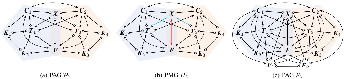
Figure 4 demonstrates why new rules were needed. In (a), if we introduce knowledge that \(C_1\) causes \(X\) and \(X\) causes \(C_2\), logically there must be an edge \(X \to F\). However, existing rules (like \(\mathcal{R}_{12}\)) wouldn’t catch this, leading to the contradiction shown in (b) where an invalid unshielded collider is formed.

To fix this, the authors propose three new rules: \(\mathcal{R}_{14}\), \(\mathcal{R}_{15}\), and \(\mathcal{R}_{16}\).

One key concept for these rules is determining if one node is “prior to” another relative to a central node \(X\).

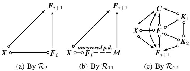
Figure 5 illustrates this “prior to” concept. It essentially checks for chains of influence. If \(F_{i+1}\) causes \(X\), does that force \(F_i\) to also cause \(X\) via rules like \(\mathcal{R}_2\) or \(\mathcal{R}_{11}\)? By formalizing this, the new rules can detect necessary orientations that previous sets missed.

The Algorithm in Action

With the new logic in place, MAGLIST-POLY operates using two nested loops:

1. Outer Loop: Picks a vertex \(X\) that still has uncertain edges (circles).
2. Inner Loop: Enumerates circles at \(X\) one by one.

• It guesses an orientation (e.g., \(X \to A\)).
• It applies the Locally Complete Orientation Rules to update the graph.
• It recurses to the next circle at \(X\).

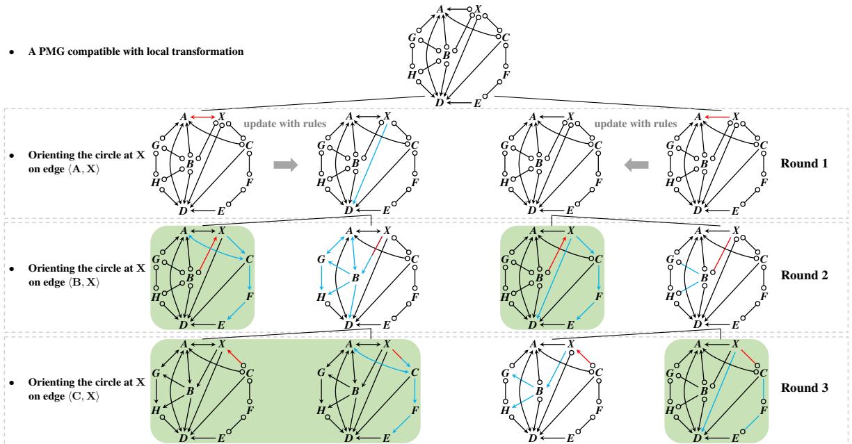
Figure 6 visualizes this inner loop.

• Round 1: We focus on the edge between \(X\) and \(A\). We make a guess (red arrow). We apply rules (blue arrows) to update the rest of the graph.
• Round 2: We move to the edge between \(X\) and \(B\), guess, and update.
• Round 3: We move to \(X\) and \(C\).

Notice the shaded graphs. These represent valid states where all circles at \(X\) are resolved. These are passed back to the outer loop.

Comparing the Approaches

It is helpful to contrast this with the previous method.

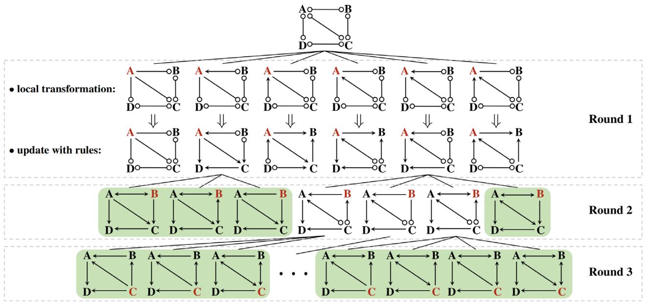
In Figure 10 (Old Method), the algorithm takes a graph and generates all valid local structures for node A, then node B, etc. It does “heavy lifting” at every step. In contrast, the new method (Figure 6) takes smaller, lighter steps, ensuring that the time between discovering valid graphs remains short.

Experimental Results: Polynomial vs. Exponential

Does this theoretical improvement matter in practice? The experiments suggest a resounding “yes.”

The authors compared MAGLIST-POLY against the old MAGLIST and a baseline BRUTE-FORCE approach. They measured the time taken to list MAGs as the graph size (\(d\)) and density (\(\rho\)) increased.

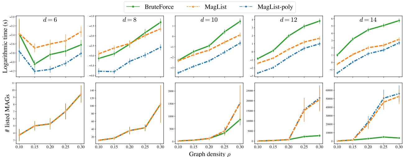
Figure 9 tells the story. Look at the top row (Logarithmic time):

• Green line (Brute Force): Explodes immediately.
• Orange line (MagList): Performs okay but spikes at specific densities.
• Blue line (MagList-Poly): The winner. Even as the graph size (\(d\)) increases to 14 nodes, the runtime remains significantly lower and more stable than the alternatives.

This confirms that avoiding the \(2^d\) enumeration allows the algorithm to handle larger, denser causal graphs efficiently.

A Note on Completeness

The paper concludes with a fascinating theoretical observation. While the proposed rules are locally complete (enough to make the algorithm work), they are not globally complete for general background knowledge.

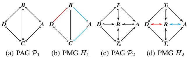
Figure 8 provides counterexamples. In (b), knowing \(D \to B\) logically implies \(C - A\), but even the new rules (\(\mathcal{R}_{14}-\mathcal{R}_{16}\)) cannot derive this. This highlights that while we have solved the polynomial delay problem, the quest for a perfect set of rules for all causal inference scenarios remains an open mathematical challenge.

Conclusion

MAGLIST-POLY represents a crucial step forward in causal discovery. By breaking down the complex problem of enumerating causal graphs into smaller, single-edge decisions—and supporting those decisions with robust new logical rules—we can now explore the space of hidden variable models much faster.

For students and researchers, this means that tools for causal experimental design and effect estimation will become more scalable, allowing us to tackle larger, more complex systems in biology, economics, and beyond.

Key Takeaways

• PAGs represent a class of possible causal graphs with hidden variables. Listing these graphs is essential for analysis.
• Previous methods suffered from exponential delay because they tried to solve local structures all at once.
• MAGLIST-POLY achieves polynomial delay by using Singleton Background Knowledge (orienting one edge at a time).
• This approach requires new Locally Complete Orientation Rules to ensure validity without exhaustive search.
• While efficient, the search for a truly complete set of orientation rules for all scenarios continues.