Introduction

Graph Neural Networks (GNNs) have revolutionized how we handle data. From predicting protein structures to recommending new friends on social media, GNNs excel at leveraging the connections between data points. But there is a massive elephant in the room: Privacy.

Real-world graphs—like social networks or financial transaction webs—are often packed with sensitive personal information. We want to train models on this data to solve useful problems, but we cannot compromise the privacy of the individuals who make up the graph.

The gold standard for privacy today is Local Differential Privacy (LDP). In an LDP setup, users add noise to their own data before it ever leaves their device. The server only sees the noisy version. While this is great for privacy, it is often catastrophic for utility. When you add enough noise to protect a user, the data becomes so distorted that a GNN struggles to learn anything useful.

So, how do we balance rigorous privacy with high model performance?

In this post, we are diving deep into a research paper that proposes UPGNET (Utility-Enhanced Private Graph Neural Network). This framework tackles the noise problem head-on. By mathematically analyzing why LDP hurts GNNs, the researchers developed a two-stage cleaning process involving Node Feature Regularization (NFR) and a High-Order Aggregator (HOA).

If you are a student or practitioner interested in the intersection of Deep Learning and Privacy, this paper offers a blueprint for making private AI actually usable.

The Privacy-Utility Tug of War

To understand UPGNET, we first need to understand the environment it operates in.

The Scenario

Imagine a cloud server wants to train a GNN for node classification (e.g., classifying users as “bots” or “humans”). The users possess sensitive feature vectors (\(\mathbf{x}\)), such as browsing history or profile details.

In a standard centralized setting, users would upload \(\mathbf{x}\) directly to the server. But in a Locally Private setting, users don’t trust the server (or the server wants to limit its liability). Instead, each user runs a perturbation mechanism \(\mathcal{M}\) on their device.

\[ \mathbf{x} \xrightarrow{\text{LDP}} \mathbf{x}' \]

The user sends the noisy \(\mathbf{x}'\) to the server. The server collects these noisy vectors and the graph structure (edges) to train the model.

The Problem: Low Utility

The problem is that existing LDP protocols for node features are destructive. Because feature vectors are often high-dimensional, the “privacy budget” (\(\epsilon\)) has to be split across many dimensions. This means each specific attribute gets very little budget, resulting in massive noise injection.

When the server tries to aggregate this noisy data using a standard GNN, the results are often poor.

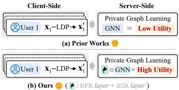
As illustrated in Figure 1, prior works (a) typically feed the noisy data directly into a GNN, leading to a “sad face” outcome—low utility. The UPGNET approach (b) inserts a specialized processing block—comprising the NFR and HOA layers—before the GNN, effectively recovering the signal from the noise.

The Root Cause: Why does LDP break GNNs?

The researchers didn’t just guess a solution; they started with a theoretical analysis of the error. They modeled the pipeline in three stages: Perturbation (client-side), Calibration (server-side adjustment), and Aggregation (GNN message passing).

The critical question is: What factors drive the “Estimation Error”? This error is the difference between the embedding the GNN should have calculated (using clean data) and the one it actually calculated (using noisy data).

Using Bernstein’s inequality, the authors derived a bound for this error.

Let’s look closely at the equation above. The maximum error (\(\xi\)) is proportional to:

\[ \mathcal{O}\left( \frac{\sqrt{d \log(d)}}{\epsilon \sqrt{|\mathcal{N}(v)|}} \right) \]

If we strip away the constants, we are left with two key levers that control the error:

1. Feature Dimension (\(d\)): The error grows as the number of features increases. High-dimensional data is harder to privatize because the noise overwhelms the sparse signals.
2. Neighborhood Size (\(|\mathcal{N}(v)|\)): The error shrinks as the neighborhood size increases. This makes intuitive sense: if you average the noisy features of 100 neighbors, the noise tends to cancel out more effectively than if you only average 2 neighbors.

The Insight: To fix private graph learning, we must effectively reduce the feature dimension and increase the effective neighborhood size.

The Solution: UPGNET

Based on that analysis, the authors propose UPGNET. It is a framework that sits between the noisy data and your GNN model. It consists of two plug-and-play layers designed specifically to manipulate those two variables (\(d\) and \(|\mathcal{N}(v)|\)).

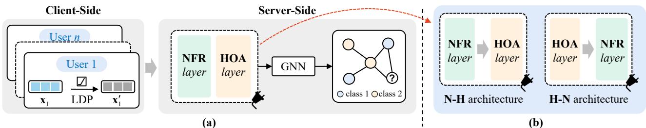
As shown in Figure 2, UPGNET can be arranged in two architectures: H-N (HOA followed by NFR) or N-H (NFR followed by HOA). Let’s break down the two core components.

Component 1: Node Feature Regularization (NFR)

Target: Reducing Effective Feature Dimension (\(d\))

Standard LDP mechanisms add noise to every dimension. If a user has a feature vector of length 1,000, but only 10 features are non-zero, the LDP mechanism still perturbs the zeros, turning a sparse vector into a dense vector of noise.

The Node Feature Regularization (NFR) layer aims to denoise this vector by inducing sparsity. It relies on a classic technique in machine learning: \(L_1\)-regularization.

The goal is to find a cleaner representation of the node features that balances fidelity to the noisy input with sparsity. The researchers formulate a loss function combining the distance from the noisy input and an \(L_1\) penalty (which forces small values to zero).

By solving this optimization problem using Proximal Gradient Descent, they derive a closed-form solution that acts as a Soft Thresholding operator.

Look at the equation above. For every feature \(i\), the new value is calculated by taking the noisy value \((\mathbf{x}'_v)_i\) and subtracting a threshold \(\mu\).

• If the noisy value is smaller than \(\mu\), it gets clamped to 0.
• If it is larger, it is reduced by \(\mu\).

This effectively acts as a gatekeeper. Since LDP noise usually manifests as random values scattered around zero, this “feature selection” step wipes out the pure noise dimensions (reducing the effective \(d\)) while preserving the strong signals that exceed the noise floor.

Component 2: High-Order Aggregator (HOA)

Target: Expanding Effective Neighborhood Size (\(|\mathcal{N}(v)|\))

The theoretical analysis showed that larger neighborhoods reduce error. However, most real-world graphs are sparse; nodes often have very few immediate neighbors.

A naive solution is to just stack many GNN layers to aggregate from neighbors of neighbors (multi-hop). This is often called Simple K-hop Aggregation (SKA). The problem with SKA is Over-smoothing.

The Over-smoothing Trap

As you aggregate over more and more hops (K increases), the representations of all nodes in the graph start to look identical. They converge to a global average. In a privacy setting, this is even worse because the noise spreads everywhere.

The researchers analyzed this using Dirichlet Energy, a metric that measures how distinct node embeddings are from their neighbors. They found that standard aggregation causes this energy to drop to zero (total smoothness) very quickly.

The HOA Algorithm

The High-Order Aggregator (HOA) solves this by using a personalized aggregation scheme. Instead of treating a 10-hop neighbor the same as a 1-hop neighbor, it maintains a strong link to the local structure.

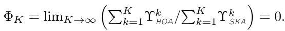
The math above proves that the ratio of Dirichlet energy in HOA vs. SKA approaches zero, meaning HOA is far more resistant to the unchecked energy decay (over-smoothing) seen in standard aggregation.

In simple terms: HOA allows the model to look far away (large \(K\)) to gather enough data points to cancel out the privacy noise, without washing out the unique features of the central node.

Experiments and Results

Does UPGNET actually work? The authors tested it on standard datasets like Cora, Citeseer, LastFM, and Facebook, comparing it against state-of-the-art private GNN methods (LPGNN, Solitude).

1. Overall Performance

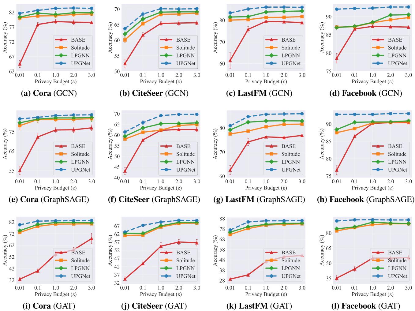
Figure 3 shows the test accuracy vs. Privacy Budget (\(\epsilon\)). Remember, a lower \(\epsilon\) means stricter privacy (more noise).

• Blue Circles (UPGNET) are consistently at the top.
• Look at Graph (c) LastFM: At strict privacy levels (\(\epsilon=0.1\)), UPGNET maintains significantly higher accuracy than the baselines (LPGNN and Solitude), which nearly collapse.
• On the Facebook dataset (Graphs d, h, l), UPGNET performs almost as well as the non-private baseline, effectively solving the privacy cost for that dataset.

2. Does NFR really help?

The researchers took standard perturbation mechanisms (like the Piecewise Mechanism, PM, and Multi-Bit Mechanism, MBM) and simply added the NFR layer to them.

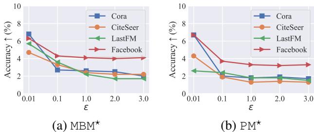
Figure 5 visualizes the “lift” provided by NFR. The curves show the improvement in accuracy.

• Notice that the improvement is highest when \(\epsilon\) is low (left side of x-axis).
• This confirms that when noise is highest, the “denoising/thresholding” effect of NFR is most valuable.

3. Does HOA really solve Over-smoothing?

This is perhaps the most interesting result. They compared HOA against the standard Simple K-hop Aggregation (SKA) while increasing the number of hops (\(K\)).

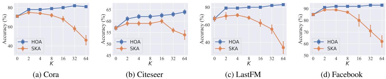
In Figure 6, look at the Orange Lines (SKA). As \(K\) gets larger (moving right), accuracy crashes. This is over-smoothing in action; the model is blurring everything together. Now look at the Blue Lines (HOA). The accuracy keeps climbing or stays stable even at \(K=64\). This proves that HOA successfully expands the neighborhood to cancel noise without destroying the signal structure.

4. Heterophilic Graphs

Most GNNs assume “homophily” (friends are similar). But what about graphs where connected nodes are different (heterophily)?

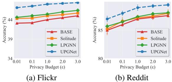
Figure 7 shows results on Flickr and Reddit (heterophilic datasets). UPGNET maintains its lead here as well. Because HOA preserves the Dirichlet energy (the difference between neighbors), it prevents the model from averaging out the distinct features of connected but dissimilar nodes.

Conclusion

The paper “Going Deeper into Locally Differentially Private Graph Neural Networks” provides a comprehensive diagnosis of why privacy hurts GNNs: too many dimensions and too few neighbors.

By introducing UPGNET, the authors offer a robust solution:

1. NFR acts as a filter, using \(L_1\)-regularization to strip away noise in high-dimensional space.
2. HOA acts as a telescope, allowing the node to gather denoising information from distant neighbors without suffering from the blurriness of over-smoothing.

For students and researchers, this work highlights the importance of aligning your privacy defense with the specific mathematical properties of your data. We cannot simply add noise and hope for the best; we need architectural changes—like NFR and HOA—to recover the utility we care about.

UPGNET demonstrates that with the right post-processing, we don’t have to choose between protecting user data and building smart models. We can do both.

---