Introduction

In the way humans learn, there is a distinct difference between “knowing what a cat is” and “knowing what a cat is not.” When you visualize a cat, you are identifying a specific set of features—whiskers, pointed ears, a tail. You do not define a cat by looking at the entire universe and subtracting dogs, cars, and trees.

However, traditional machine learning classification often works the latter way. A standard neural network classifier, when trained to distinguish between two classes (say, Class 1 and Class 2), typically slices the entire feature space into two regions. Every single point in the universe of data must belong to either Class 1 or Class 2.

This leads to a fundamental problem: What happens to the empty space? What happens to the vast regions of data that look nothing like a cat or a dog? In standard networks, these regions are arbitrarily assigned to one of the classes, leading to overconfidence on nonsense inputs.

The research paper “Discovering a Zero (Zero-Vector Class of Machine Learning)” proposes a fascinating shift in perspective. The authors suggest that we should stop thinking of classes as merely labels and start treating them as vectors in a mathematical vector space.

By rigorously defining this vector space, the researchers stumbled upon a profound question: If classes are vectors, what is the Zero-Vector? What is the mathematical equivalent of “nothing” in the context of machine learning classes?

The answer they found—the Metta-Class—provides a new framework for learning “true” data manifolds, enabling neural networks to say “I don’t know” and allowing for modular, continual learning.

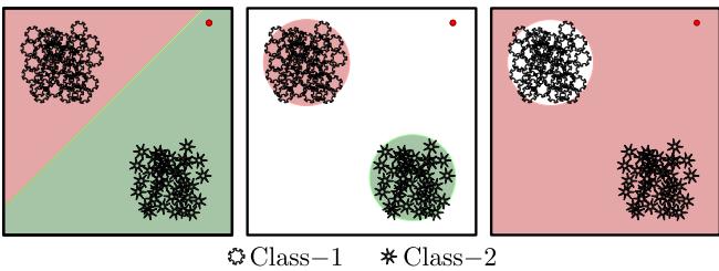
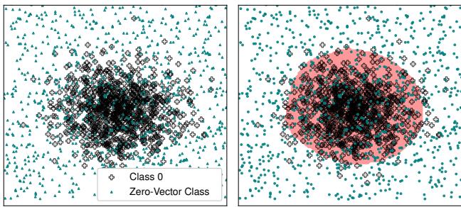
As shown in Figure 1, standard networks (far-left) dichotomize the whole space. The goal of this research (middle) is to learn tight, accurate regions that represent the true nature of the data.

1. Background: The Logit Landscape

To understand how we get to a “Zero-Vector,” we first need to redefine what a “class” actually is in the context of a neural network.

When a neural network processes an image, the final layer outputs raw numbers called logits. These logits are usually passed through a Softmax or Sigmoid function to get probabilities. The researchers propose looking at the logits themselves as functions describing the class.

The Valid Equivalence Set

A class isn’t defined by a single equation. If you have a probability density function (PDF) describing your data, \(f(x)\), you decide if a point belongs to that class by checking if \(f(x)\) is higher than some threshold.

But here is the catch: many different mathematical functions can result in the exact same classification decision. If you scale the function by a constant or shift it, the decision boundary might remain the same if you adjust the threshold accordingly.

The authors define the Valid Equivalence Set (represented as \([f(x)]\)) as the set of all logit equations that classify the data correctly for a given distribution.

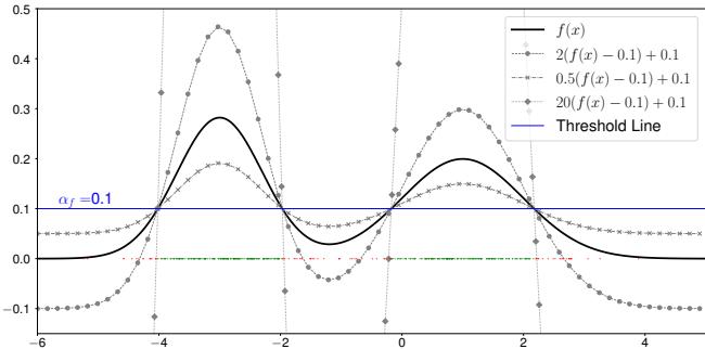
As illustrated in Figure 2, multiple curves (solid, dotted, dashed) can all successfully classify the data (the peaks) against a threshold line. In this framework, the “Class-Vector” is not just one function, but this entire set of valid functions.

2. The Core Method: Building a Vector Space

The heart of this paper is the construction of a Vector Space for these classes. For a set of objects to form a vector space, you need two primary operations: Addition and Scalar Multiplication. The authors define these operations based on set theory concepts.

2.1 Addition as Union

What happens when you add two classes together? Intuitively, “Class A + Class B” should result in a super-class that contains both A and B.

Mathematically, if \([f(x)]\) is the vector for Class-F and \([g(x)]\) is the vector for Class-G, their addition is defined by the union of their probability distributions.

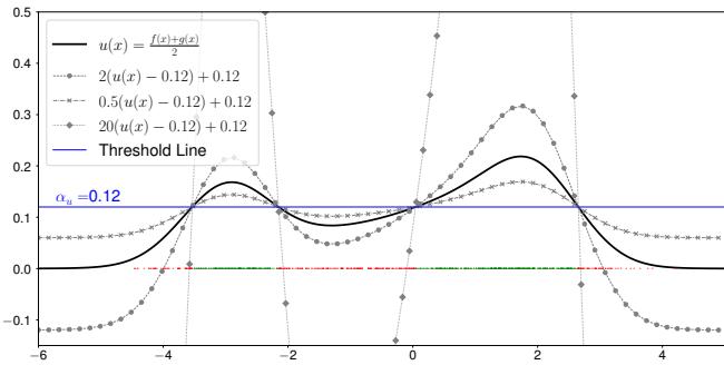
Figure 4 shows the result of combining two classes. The new function \(u(x)\) captures the peaks of both original distributions.

The mathematical definition is elegant in its simplicity:

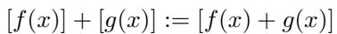
This means the vector sum of two class equivalence sets is the equivalence set of their sum.

2.2 Scalar Multiplication as Complement

Scalar multiplication in this framework is fascinating because it relates to the complement of a set (the “NOT” operation).

If you multiply a class vector by a negative scalar (specifically -1), you invert the function. This effectively flips the decision boundary. The region that was previously “positive” (inside the class) becomes “negative,” and the region that was outside becomes inside.

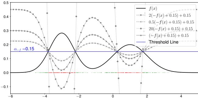
Figure 5 visualizes this concept. The peaks become valleys. This allows the framework to handle logical operations like “NOT Class A.”

2.3 The Discovery of the Zero-Vector (The Metta-Class)

Now we arrive at the pivotal discovery. In any linear vector space, there must exist an Additive Identity—a zero vector. For any vector \(v\), there must be a vector \(0\) such that:

In the context of our classes:

What kind of probability distribution, when added to another distribution, leaves the classification decision boundaries unchanged?

The authors perform a rigorous derivation involving limits. They define the normalization constant of the zero vector’s PDF over a volume \(\mathcal{V}\) as the volume approaches infinity.

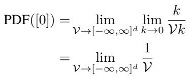
The result of this derivation is profound: The PDF of the Zero-Vector is a Uniform Distribution.

Why does this make sense? Imagine you have a mountain (your data class) on a flat plain. If you raise the entire ground level by a constant amount (adding a uniform distribution), the mountain is still a mountain. The relative decision of “is this point on the mountain or not?” remains unchanged, provided you adjust your threshold.

The authors name this Zero-Vector class the Metta-Class.

What is the Metta-Class in practice?

It is noise. It is a distribution where data is uniformly spread across the entire finite volume of the feature space.

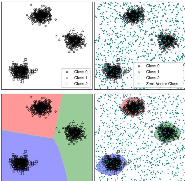
Figure 6 illustrates this perfectly:

• Top-Left: Standard data clusters.
• Top-Right: The data clusters plus the Metta-Class (the teal dots scattered everywhere).
• Bottom-Right: When a network is trained with this “Zero” class included, the decision boundaries (the colored regions) wrap tightly around the actual data. The empty space is correctly identified as “Zero” (background/noise).

3. Applications of the Zero-Vector

The discovery of the Metta-Class is not just a mathematical curiosity; it unlocks several powerful applications that solve long-standing problems in deep learning.

3.1 Clear Learning (True Manifold Learning)

Standard classifiers suffer from “open space risk”—they confidently classify noise as a known class because their boundaries extend to infinity.

By including the Metta-Class (uniform noise) during training, we force the network to distinguish between “Specific Class” and “Random Noise.” The network learns to push the logits of the class up only where the data actually exists.

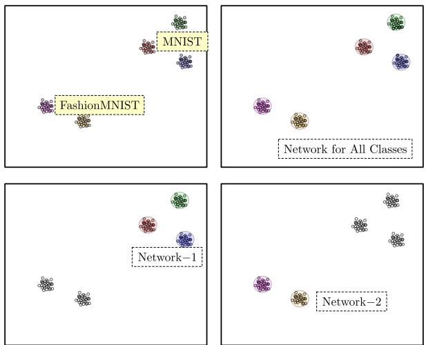
Figure 13 demonstrates this capability.

• Network-1 and Network-2 (Bottom): These networks are trained on specific datasets (MNIST and FashionMNIST) plus the Metta-Class. Notice how the boundaries (pink and green) are distinct and tight. They do not claim the whole space.
• Top-Right: Because the boundaries are tight, you can overlay them. This enables modularity.

3.2 Unary (Uni-Class) Classification

Can you train a neural network on a single class? Usually, the answer is no—you need a negative class to distinguish against.

With the Metta-Class, the answer is yes. You treat the Metta-Class as the “negative” class. You train a binary classifier: Class X vs. The Universe (Zero-Vector).

As shown in Figure 7, this allows for Unary Classifiers. You can build a separate neural network for “Cats,” another for “Dogs,” and another for “Cars,” all trained in isolation.

3.3 Continual Learning without Catastrophic Forgetting

In standard AI, if you train a network on Task A, then train it on Task B, it forgets Task A. This is because the weights are overwritten to minimize the loss for B, often destroying the boundaries set for A.

The Zero-Vector framework offers a solution: The Repository Approach. Because each Unary Classifier learns tight boundaries and treats everything else as “Zero,” you can simply add new classifiers to a repository without retraining the old ones.

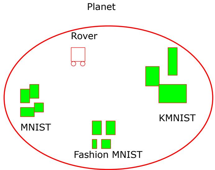
The authors use the analogy of a Rover on a Planet (Figure 43). The rover encounters new data types sequentially. It trains a new “Unary Network” for each new type it finds. Because the networks don’t fight over the empty space, they can coexist.

3.4 Logical Set Operations

Since the vector space operations correspond to set operations, we can perform logic on trained neural networks.

• Union (\(A \cup B\)): Add the logit vectors.
• Intersection (\(A \cap B\)): Can be derived from union and complement.
• Complement (\(A^c\)): Multiply by scalar -1.

This allows us to answer complex queries like “Show me data that is Class A AND NOT Class B” by simply combining the outputs of the unary networks mathematically.

4. Experiments and Metrics

To prove the effectiveness of this method, the authors needed new metrics. Standard accuracy isn’t enough because a classifier that claims the whole universe can still have 100% accuracy on the test set (if the test set only contains class data).

4.1 New Metrics: Occupancy and Purity

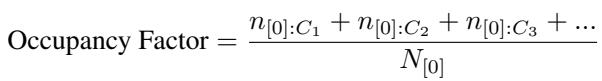
• Occupancy Factor: Measures how much “volume” the classifier claims. We want this to be low (tight fit). It is calculated by testing how many noise (Metta-Class) points are misclassified as the positive class.

• Purity Factor: Measures how “pure” the claimed region is. Inside the decision boundary, is it mostly real data?

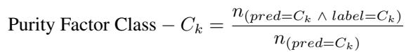
Figure 15 and Figure 16 below visualize why these metrics are necessary.

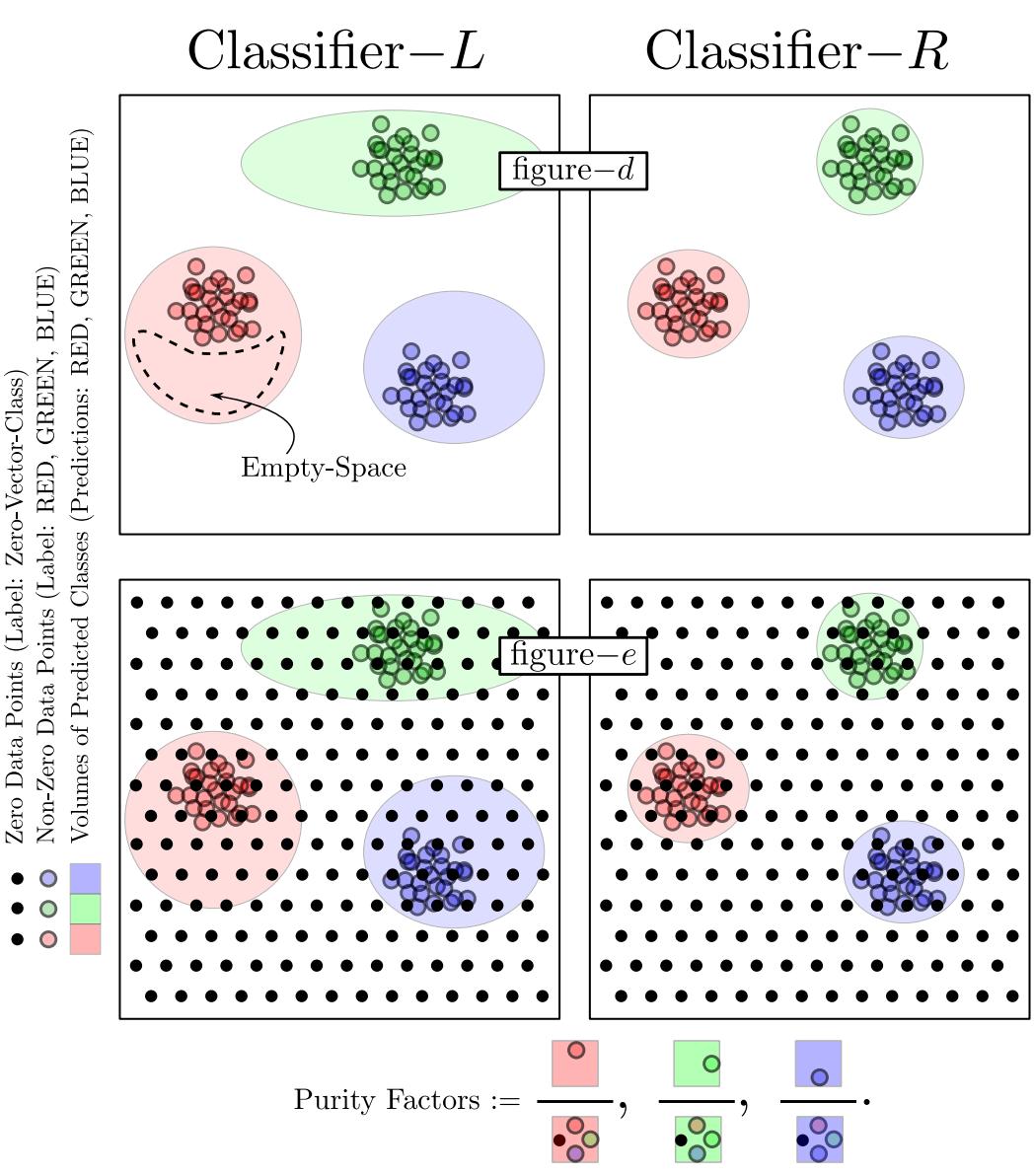
In Figure 15, Classifier-L claims too much space (high Occupancy). Classifier-R is tighter (low Occupancy). In Figure 16, Classifier-L includes empty regions (low Purity). Classifier-R hugs the data (high Purity).

4.2 Results on MNIST

The researchers trained Unary Classifiers on MNIST digits using the Metta-Class.

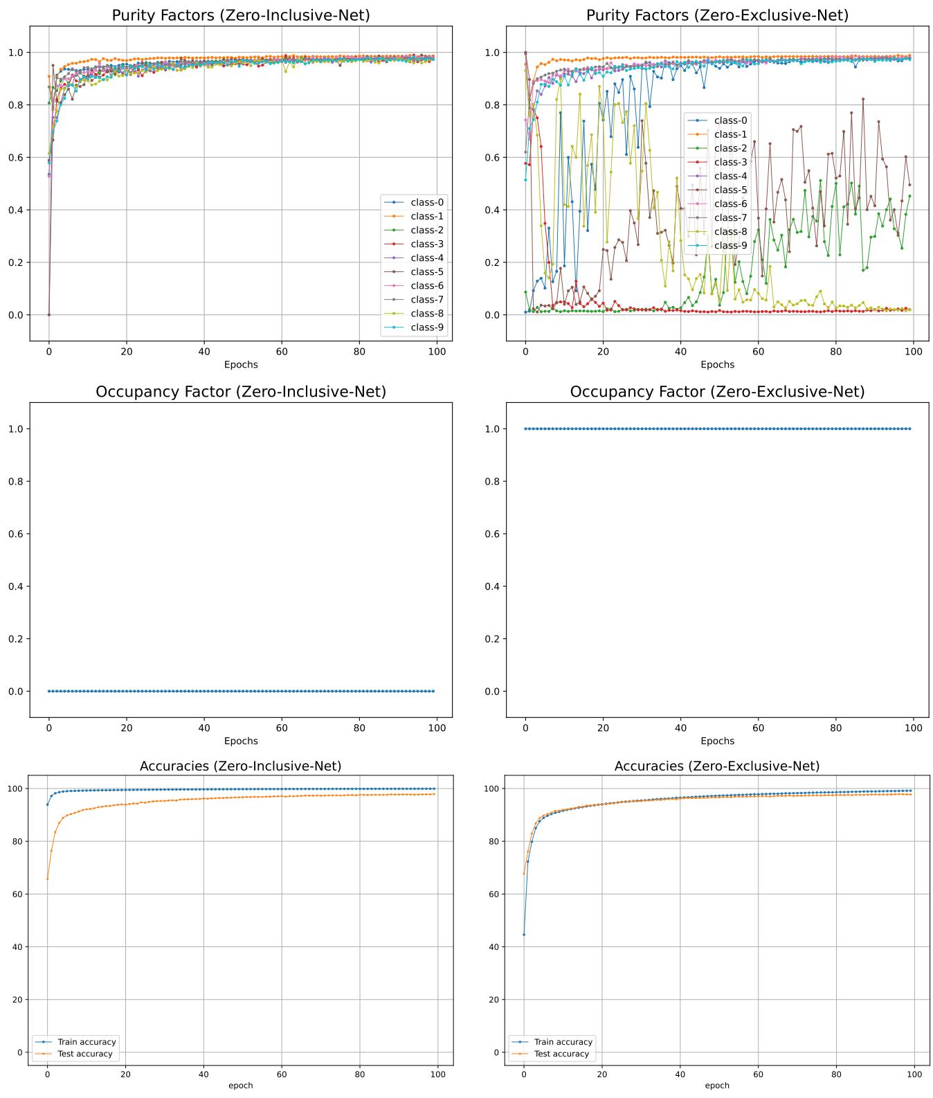
Figure 18 presents the results:

• Top Row (Purity): The Zero-Inclusive Network (left) achieves consistently high purity for all classes. The standard network (right) is erratic.
• Middle Row (Occupancy): The Zero-Inclusive Network has near-zero occupancy (it only claims the necessary space). The standard network has an occupancy of 1.0 (it claims the whole space).
• Bottom Row (Accuracy): Crucially, the test accuracy remains comparable. We get the same accuracy, but with much tighter, more meaningful boundaries.

4.3 Generative Capabilities

Because the network learns the true manifold (the actual shape of the data distribution) rather than just a wall between classes, the gradients of the logits point towards the “center” of the class.

This allows for data generation. By starting with random noise and performing gradient ascent on the class logit, the authors generated new images.

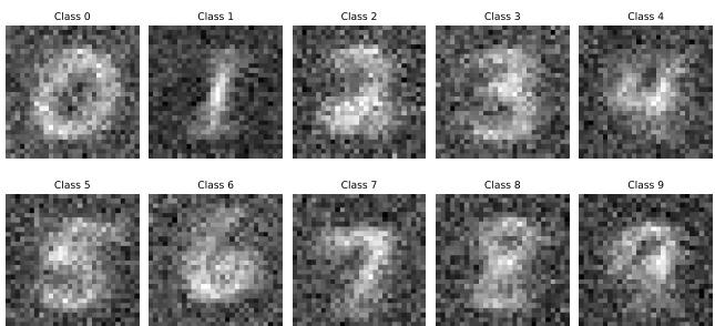
Figure 9 shows digits generated solely by following the gradients of a Unary Classifier trained against the Metta-Class.

5. Conclusion & Implications

The paper “Discovering a Zero” bridges a gap between abstract linear algebra and practical deep learning. By formalizing classes as vectors, the authors deduced that the Zero-Vector is uniform noise.

This insight allows us to:

1. Stop “Split Brain” AI: Instead of one giant network trying to learn everything (and forgetting old things), we can build modular repositories of Unary Classifiers.
2. Learn True Boundaries: By training against “nothing” (the Metta-Class), we force the network to define “something” accurately.
3. Combine Logic and Learning: The vector space allows for Boolean operations on learned classes.

While the authors note that scaling to high-dimensional datasets like CIFAR-10 presents computational challenges (requiring larger networks to maintain the same purity), the theoretical framework offers a refreshing “first-principles” look at classification. It suggests that to truly understand the data, our machines must first understand the empty space that surrounds it.

In the quest to build intelligent systems, it turns out that discovering “Zero” might be just as important for machines as it was for mathematics.