Can We Teach RTL Models Physics? Inside the RTLDistil Framework

In the world of modern chip design, speed is everything—not just the clock speed of the final processor, but the speed at which engineers can design it. This creates a fundamental tension in Electronic Design Automation (EDA). On one hand, you want to know if your design meets timing constraints as early as possible (at the Register-Transfer Level, or RTL). On the other hand, you can’t really know the timing until you’ve done the physical layout, which includes placing components and routing wires.

This creates a massive feedback loop bottleneck. Engineers write code, synthesize it, run through a physical layout engine (which takes hours or days), and only then realize they have a timing violation. This process, often called the “Slow EDA Flow,” is a major productivity killer.

The industry solution is the “Left-Shift” paradigm: moving verification and prediction earlier in the timeline. But there is a catch. RTL code is abstract logic; it doesn’t know about wire resistance, capacitance, or physical congestion. So, how do you make an abstract RTL model predict physical realities accurately?

The answer might lie in RTLDistil, a new framework presented at the 42nd International Conference on Machine Learning. This paper proposes a clever solution: using Knowledge Distillation to transfer the “physical wisdom” of a layout-aware model into a fast, lightweight RTL model.

In this deep dive, we will explore how RTLDistil works, the architecture of its Graph Neural Networks (GNNs), and why its multi-granularity approach sets a new standard for early-stage timing prediction.

The Problem: The Abstract vs. The Physical

To understand why this research is necessary, we first need to visualize the gap between RTL and Layout.

RTL (usually written in Verilog or SystemVerilog) describes what the chip does. It defines registers, logic gates, and the flow of data. However, it treats connections as ideal, instant pathways. It ignores the physical reality that electricity takes time to travel down a wire, and that crowded areas of a chip create parasitic resistance and capacitance (RC).

The Physical Layout is the blueprint for manufacturing. It knows exactly where every flip-flop sits and how long every wire is. This allows for Static Timing Analysis (STA), the gold standard for accuracy.

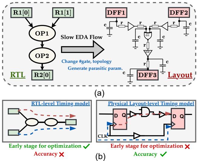
As shown in Figure 1 above, there is a stark contrast. The RTL model (left) is fast but inaccurate (marked with a red cross) because it guesses timing based on logic depth. The Physical model (right) is accurate but computationally expensive and occurs too late in the design cycle to be used for rapid iteration.

The goal of RTLDistil is to get the accuracy of the right side with the speed of the left side.

The Solution: Teacher-Student Distillation

The researchers approach this problem using Knowledge Distillation (KD). KD is a machine learning technique where a large, complex model (the Teacher) trains a smaller, simpler model (the Student) to mimic its behavior.

In the context of RTLDistil:

1. The Teacher (Layout GNN): This model sees the full physical netlist. It knows about cell drive strengths, capacitance, input/output slews, and wire delays. It is trained to be an expert on physical timing.
2. The Student (RTL GNN): This model only sees the abstract RTL graph (Simple Operator Graph, or SOG). It has no access to physical parameters during inference.
3. The Distillation: During training, the Teacher forces the Student to align its internal feature representations with the Teacher’s physical insights.

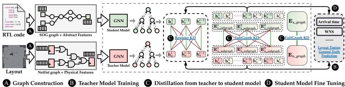
Figure 2 outlines the entire pipeline. Note that the process involves constructing graphs for both stages, training the teacher, and then distilling that knowledge through three specific levels (Node, Subgraph, and Global) into the student. Finally, the student model is fine-tuned for the actual prediction tasks.

Data Representation: A Tale of Two Graphs

The disparity between what the Teacher knows and what the Student knows is vast. The table below illustrates the features available to each model.

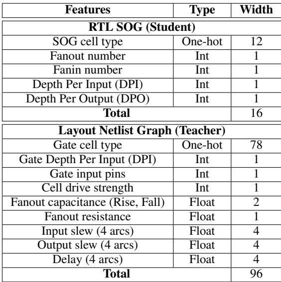
The Student (RTL) has a feature vector of size 16, consisting mostly of logical depths and fan-in/fan-out counts. The Teacher (Layout), however, operates on 96-dimensional vectors containing rich physical data like resistance, capacitance (Rise/Fall), and delay arcs.

The challenge is significant: The Student must learn to predict outcomes based on physical phenomena (like capacitance) without ever explicitly seeing the data for those phenomena.

Core Methodology: Graph Neural Networks and Propagation

Both the Teacher and Student models are built using Graph Neural Networks (GNNs), specifically Graph Attention Networks (GATs). Circuits are naturally represented as graphs where logic gates are nodes and wires are edges.

However, standard GNN propagation (aggregating neighbor information) isn’t quite enough for timing analysis. In digital circuits, timing is governed by paths. A signal accumulates delay as it moves forward, but timing constraints (slack) are often calculated by looking at the required arrival time, which propagates backward from the output.

Asynchronous Forward-Reverse Propagation

To mimic the actual physics of delay propagation and Static Timing Analysis (STA), the researchers developed a domain-specific Asynchronous Forward-Reverse Propagation strategy.

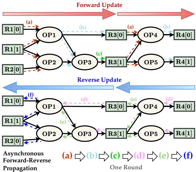
As visualized in Figure 3, the model doesn’t just update nodes in a random order.

1. Forward Pass (Red Arrows): Information flows from inputs (Source) to outputs (Sink). This mimics the accumulation of cell and wire delays (Arrival Time).
2. Reverse Pass (Blue Arrows): Information flows from outputs back to inputs. This mimics the propagation of required arrival times and slack calculation.

This bidirectional flow allows every node to understand its context: “How long has the signal taken to reach me?” (Forward) and “How much time do I have left to get the signal to the end?” (Reverse).

The mathematical update rule for a node’s feature \(h\) combines its neighbors’ features weighted by an attention mechanism \(\alpha\):

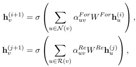
In these equations, \(\mathcal{N}(v)\) represents forward neighbors (fan-in) and \(\mathcal{R}(v)\) represents reverse neighbors (fan-out). The Teacher model runs more rounds of this propagation to capture long-path accumulation, while the Student runs fewer rounds to stay lightweight and fast.

The Secret Sauce: Multi-Granularity Distillation

If we simply trained the Student to predict the final timing number (a scalar value like “1.5ns”), it would likely overfit or fail to generalize. It needs to “think” like the Teacher, not just guess the Teacher’s answer.

RTLDistil employs Multi-Granularity Knowledge Distillation, aligning the models at three distinct structural levels. This ensures the Student learns physical dependencies at the local, regional, and global scales.

1. Node-Level Distillation (The Register)

At the finest grain, the model aligns features at specific register nodes (Flip-Flops). This ensures that for a specific register \(v\), the Student’s embedding represents the same timing criticality as the Teacher’s embedding.

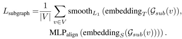
The loss function uses a smooth \(L_1\) distance metric to minimize the difference between the Teacher’s embedding (\(embedding_T\)) and the Student’s projected embedding (\(embedding_S\)):

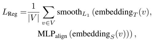
The smooth \(L_1\) loss is chosen because it is less sensitive to outliers than Mean Squared Error (\(L_2\)) and smoother near zero than absolute error (\(L_1\)):

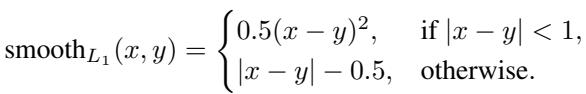
2. Subgraph-Level Distillation (The Context)

A register doesn’t exist in a vacuum; its timing is determined by the “Fan-in Cone”—the cloud of combinational logic (AND, OR, NOT gates) feeding into it.

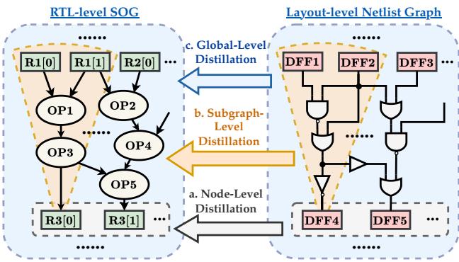
As shown in Figure 4 (b), Subgraph Distillation aggregates the embeddings of the entire fan-in cone. This forces the Student to understand the structural complexity driving the signal to the register. If the Teacher sees a high-resistance path in the layout, the Student must learn to recognize the corresponding logic topology in the RTL that caused it.

Here, \(\mathcal{G}_{sub}(v)\) represents the subgraph (fan-in cone) for node \(v\).

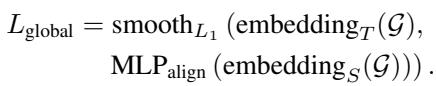
3. Global-Level Distillation (The Big Picture)

Finally, the model looks at the entire circuit graph \(\mathcal{G}\). Global distillation pools all node embeddings to form a single graph vector. This helps the Student account for chip-wide properties, such as overall congestion or clock tree characteristics, which affect timing globally.

The Total Loss Function

The training process combines all these distillation losses with the actual supervised loss (the error in predicting the Arrival Time).

The coefficients \(\alpha, \beta, \gamma\) allow the researchers to tune the importance of each granularity level. This comprehensive loss function guides the Student model to essentially hallucinate the physical parameters it cannot see, resulting in highly accurate predictions.

Experimental Results

The researchers evaluated RTLDistil on a dataset of 2,004 RTL designs, ranging from small arithmetic blocks to complex RISC-V subsystems. This diversity ensures the model isn’t just memorizing one type of circuit.

The key metrics for evaluation are:

• Arrival Time (AT): When the signal gets there.
• Worst Negative Slack (WNS): The most critical timing violation in the design.
• Total Negative Slack (TNS): The sum of all timing violations (a measure of how “bad” the overall design is).
• MAPE: Mean Absolute Percentage Error (lower is better).
• PCC: Pearson Correlation Coefficient (closer to 1.0 is better).

Comparison with State-of-the-Art

RTLDistil was compared against MasterRTL and RTL-Timer, the previous leaders in this space. The results, summarized in Table 2, are striking.

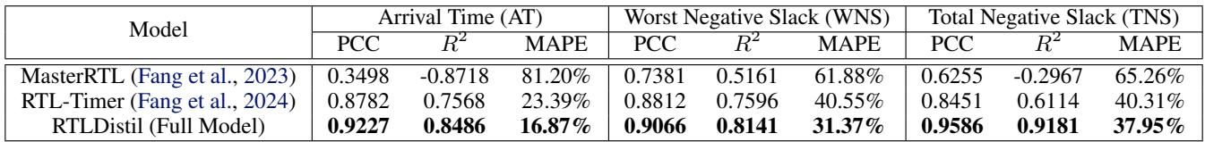
Looking at Arrival Time (AT), RTLDistil achieves a correlation (PCC) of 0.9227, significantly higher than MasterRTL (0.3498) and RTL-Timer (0.8782). Even more impressive is the error reduction: RTLDistil brings the MAPE down to 16.87%.

For Total Negative Slack (TNS), which is notoriously hard to predict because errors accumulate, RTLDistil jumps to a 0.9586 correlation, while MasterRTL struggles at 0.6255.

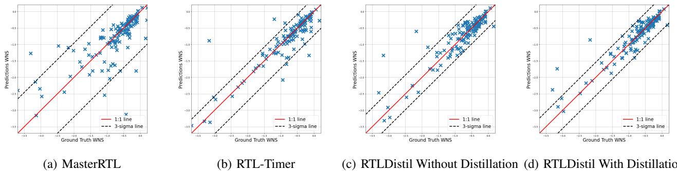
Visualizing the Correlation

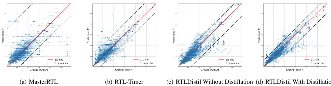
Numbers in a table are one thing, but scatter plots tell the real story. In the figures below, the X-axis is the Ground Truth (Physics) and the Y-axis is the Prediction. Ideally, all blue stars should sit perfectly on the red diagonal line.

Arrival Time (AT): In Figure 6, notice how scattered MasterRTL (a) and RTL-Timer (b) are. RTLDistil (d) shows a tight clustering along the diagonal line, indicating high precision.

Worst Negative Slack (WNS): WNS is critical because it determines the maximum clock frequency of the chip. Figure 7 shows that MasterRTL (a) has massive outliers. RTLDistil with Distillation (d) pulls those outliers in, adhering closely to the 1:1 line.

Does Distillation Really Help? (Ablation Study)

One might ask: “Is it the GNN architecture doing the work, or is it the Knowledge Distillation?” The researchers performed an ablation study to isolate the impact of the distillation process.

Table 3 compares the Teacher (the upper bound of performance) against the Student with and without distillation.

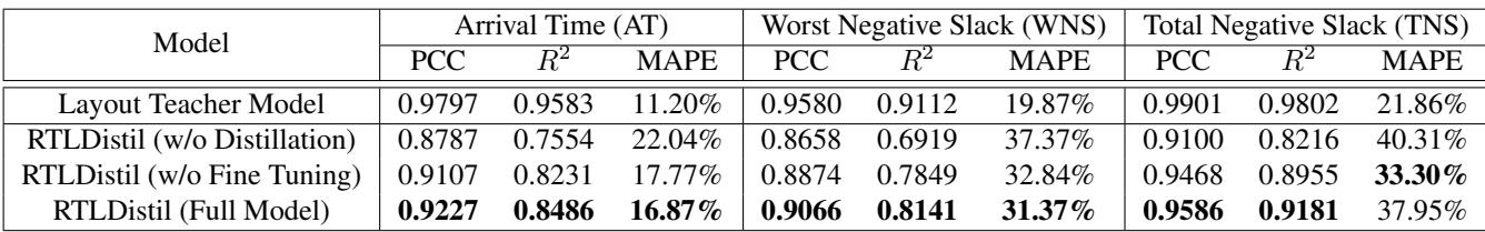
The “RTLDistil (w/o Distillation)” row shows what happens if you just train the RTL model on the labels without the Teacher’s guidance. The MAPE for Arrival Time is 22.04%. When you add the distillation and fine-tuning (Full Model), the error drops to 16.87%. This proves that the student is indeed learning “hidden” knowledge from the teacher.

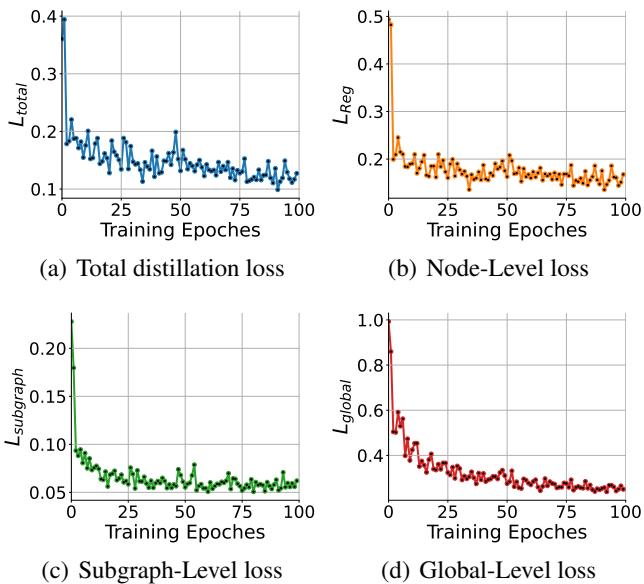
Furthermore, the training dynamics show how the model learns. Figure 5 displays the loss curves for the different granularities. You can see the Node-Level loss (b) drops quickly—registers are easy to align. The Global-Level loss (d) takes longer, suggesting it’s harder to align the overall “vibe” of the circuit, but it eventually converges.

Propagation Strategy Analysis

Finally, the team validated their “Forward-Reverse” propagation theory. Is it better than just going forward?

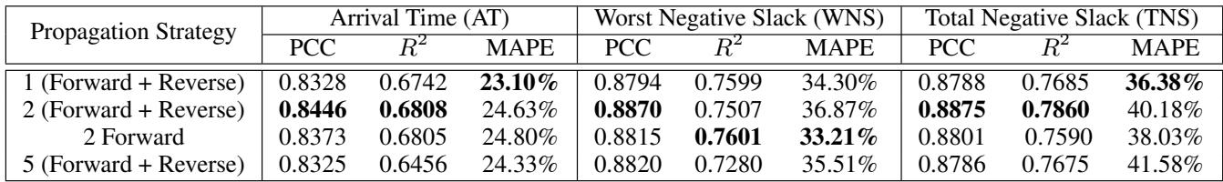
Table 5 confirms that the bidirectional approach (“2 Forward + Reverse”) beats the forward-only approach. It also highlights an interesting finding: more isn’t always better. Increasing to 5 rounds of propagation actually degraded performance slightly, likely due to overfitting or noise amplification (the “oversmoothing” problem common in GNNs).

Conclusion and Future Implications

RTLDistil represents a significant step forward in the “Left-Shift” movement of EDA. By successfully bridging the gap between the abstract RTL world and the physical Layout world, it offers a tool that is both fast enough for early-stage design exploration and accurate enough to be trusted.

The core innovation isn’t just the GNN, but the Multi-Granularity Knowledge Distillation. By forcing the RTL model to understand the circuit at the node, subgraph, and global levels, the researchers have created a model that hallucinates physical reality with surprising accuracy.

For students and researchers in EDA, this highlights the potential of AI not just to automate tasks, but to translate between different levels of abstraction. As designs become more complex and “Moore’s Law” slows down, tools like RTLDistil will be essential for squeezing maximum performance out of silicon in minimal time. The future of chip design isn’t just about better physics engines; it’s about smarter models that can learn physics from the experts.