One Size Doesn’t Fit All: Customizing Graph Foundation Models with AutoGFM

In the world of Natural Language Processing (NLP), Foundation Models like GPT-4 have revolutionized the field by providing a single, unified model capable of handling diverse tasks. The graph machine learning community has been racing to achieve a similar feat: creating Graph Foundation Models (GFMs). These models aim to share knowledge across diverse domains—from social networks to molecular structures—allowing a single model to perform node classification, link prediction, and graph classification.

However, there is a significant hurdle. Unlike text, where the structural format (sequences of tokens) is relatively consistent, graphs vary wildly. A citation network looks nothing like a protein molecule. Current GFMs typically rely on a hand-designed, fixed Graph Neural Network (GNN) architecture (like a standard GraphSAGE backbone) for all inputs.

This leads to a problem: Architecture Inconsistency. The optimal neural architecture for a social network is rarely the optimal one for a molecular graph. By forcing a single architecture on everyone, we inevitably settle for suboptimal performance.

In this post, we will dive deep into AutoGFM (Automated Graph Foundation Model), a novel approach presented at ICML 2025. This paper proposes a method to automatically customize the neural architecture for each specific graph dataset, combining the power of foundation models with the precision of Neural Architecture Search (GNAS).

The Core Problem: Architecture Inconsistency

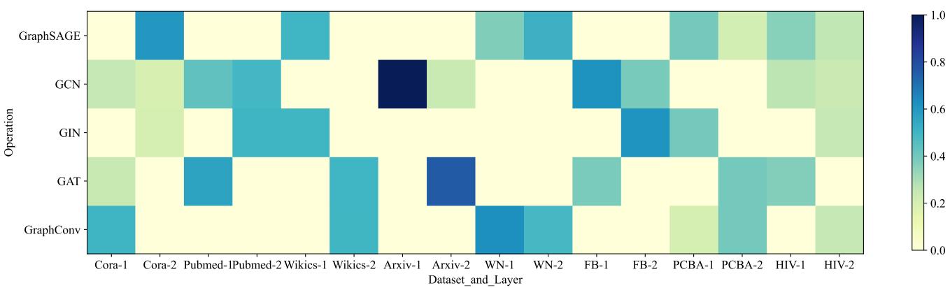
To understand why AutoGFM is necessary, we first need to visualize the problem. The researchers conducted a preliminary study testing various popular GNN architectures (GCN, GAT, GraphSAGE, etc.) across different datasets.

As shown in Figure 1, there is no single “winner.”

• GCN (Graph Convolutional Network) performs excellently on the Arxiv dataset (dark blue) but struggles on the WikiCS dataset.
• GraphSAGE is strong on Cora but weak elsewhere.

If you build a Graph Foundation Model using only GCN as your backbone, you automatically cap your performance on tasks that would have preferred an attention mechanism (GAT). This phenomenon is what the authors call Architecture Inconsistency.

Existing Graph Neural Architecture Search (GNAS) methods try to find the “best” architecture, but they typically search for a single architecture that minimizes the total loss across all training data. When that data comes from vastly different domains (as is the case for Foundation Models), the search algorithm faces optimization conflicts. It tries to satisfy divergent needs and ends up finding a “compromise” architecture that isn’t great for anyone.

The Solution: AutoGFM

The researchers propose AutoGFM, a framework that treats architecture not as a fixed global hyperparameter, but as a dynamic prediction based on the input graph’s characteristics.

The core idea is to learn a mapping function \(\pi\) that takes a graph \(\mathcal{G}\) and outputs a customized architecture \(\mathcal{A}\).

The High-Level Framework

The AutoGFM framework consists of three main components designed to handle the complexity of diverse graph data:

1. Disentangled Contrastive Graph Encoder: To figure out what architecture a graph needs, we first need to understand the graph’s properties. This encoder splits graph features into Invariant patterns (structural properties that dictate architecture) and Variant patterns (noise or task-specific data that shouldn’t influence architecture choice).
2. Invariant-Guided Architecture Customization: A “Super-Network” that uses the invariant patterns to dynamically select the best GNN operations (layers) for the specific input.
3. Curriculum Architecture Customization: A training strategy that prevents easy datasets from dominating the search process early on.

Let’s break down these components step-by-step.

Step 1: Disentangled Contrastive Graph Encoder

How do we decide which architecture is best for a given graph? The authors argue that we need to look at the graph’s intrinsic properties from an “invariant” perspective.

They assume that graph data consists of two parts:

1. Invariant Patterns (\(Z_I\)): These are stable features associated with the optimal architecture. For example, whether a graph is homophilic (neighbors are similar) or heterophilic is an invariant pattern that strongly suggests whether we should use GCN or a different operator.
2. Variant Patterns (\(Z_V\)): These are features correlated with the specific data instance but irrelevant or noisy regarding the architecture choice.

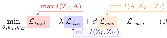
The goal is to maximize the mutual information between the invariant patterns \(Z_I\) and the architecture \(A\), while minimizing the interference from variant patterns \(Z_V\). The optimization objective looks like this:

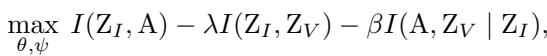
Here, the model tries to:

• Maximize the link between \(Z_I\) and Architecture \(A\).
• Minimize the overlap between \(Z_I\) and \(Z_V\) (disentanglement).
• Ensure that given \(Z_I\), the architecture \(A\) is independent of \(Z_V\).

The Encoder Architecture

To achieve this separation, the model uses two separate GNN channels. Given a subgraph (defined as a “Node of Interest” or NOI-graph), the encoder processes it through two parallel streams:

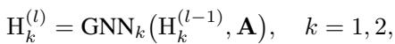
Followed by a Multi-Layer Perceptron (MLP) and a pooling (Readout) function to get the graph-level representations:

Contrastive Learning

To force these representations to actually capture meaningful differences, AutoGFM uses Contrastive Learning. The idea is simple: graphs from the same domain/task likely share similar architectural needs (similar \(Z_I\)), while graphs from different domains should be pushed apart in the embedding space.

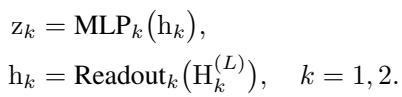
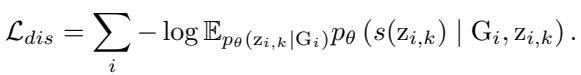
The model uses a loss function that pulls the invariant representation \(z_{i,k}\) closer to a “prototype” \(p_k\) of its cluster, while pushing it away from others:

Furthermore, to ensure the invariant patterns (\(Z_I\)) are distinct from the variant patterns (\(Z_V\)), the model employs a discriminative task. This forces the encoder to recognize that \(Z_I\) and \(Z_V\) represent different aspects of the graph.

Step 2: Invariant-Guided Architecture Customization

Once we have the invariant representation \(Z_I\), we need to translate it into an actual Neural Network architecture. AutoGFM uses a Weight-Sharing Super-Network.

Imagine a giant GNN layer that contains all possible operations at once—GCN, GAT, GIN, etc. The output of this layer is a weighted sum of all these operations.

Here, \(\alpha_{l,i}\) represents the probability (or weight) of selecting operation \(i\) at layer \(l\).

The Predictor

Instead of learning a fixed \(\alpha\) for the whole dataset (as standard NAS does), AutoGFM uses a Predictor (\(\psi_I\)) that takes the invariant graph representation \(z\) and outputs the weights \(\alpha\).

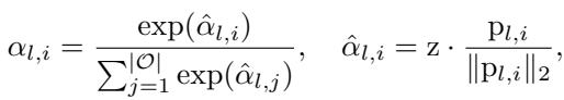
If the graph representation \(z\) is close to the learnable prototype \(p_{l,i}\) for a specific operation (say, GAT), then the weight for GAT increases. This effectively “routes” the graph to the correct neural architecture.

Shielding from Variant Patterns

A key innovation here is preventing the “Variant” (noisy) patterns from messing up the architecture prediction. The authors propose a clever training trick using an Auxiliary Predictor (\(\psi_E\)).

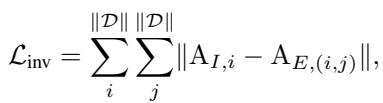
They generate two architecture predictions:

1. \(A_I\): Predicted using only the invariant patterns \(Z_I\).
2. \(A_E\): Predicted using a fusion of \(Z_I\) and the variant patterns \(Z_V\).

The goal is to make \(A_I\) and \(A_E\) identical. If the architecture prediction changes when we add the variant patterns (\(Z_V\)), it means our predictor is being influenced by noise. By minimizing the difference between these two predictions, the model learns to ignore \(Z_V\) and rely solely on \(Z_I\).

Step 3: Curriculum Architecture Customization

Training a Foundation Model involves diverse datasets. Some are “easy” (easy to fit with almost any GNN), and some are “hard.”

If we train naively, the super-network will likely converge on operations that work well for the easy, dominant datasets early in the training process. The operations needed for the harder, more complex datasets might be starved of gradients and never learned. This is the Data Domination phenomenon.

To fix this, AutoGFM introduces a Curriculum mechanism. It encourages diversity in the architecture choices during the early stages of training.

It calculates the coefficient of variation (CV) of the selected operations across the different datasets.

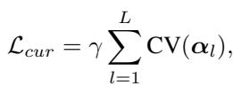
By adding this term to the loss function, the model is penalized if it selects the same operations for everyone. As training progresses (controlled by a pacing parameter \(\gamma\)), this penalty is reduced, allowing the model to settle on the optimal (potentially similar) architectures if necessary. But the initial “forced diversity” ensures all operations get a fair chance to be learned.

The Final Objective

The complete training objective combines the task loss (classification accuracy), the disentanglement loss (splitting \(Z_I\) and \(Z_V\)), the invariance loss (consistency between predictors), and the curriculum loss:

Experiments and Results

Does this complex machinery actually pay off? The authors tested AutoGFM on a variety of datasets including citation networks (Cora, PubMed), knowledge graphs (WN18RR), and molecular graphs (HIV, PCBA).

Comparison with Baselines

AutoGFM was compared against:

• Vanilla GNNs: Standard GCN, GAT, GIN.
• Self-Supervised Methods: GraphMAE, BGRL.
• Other GFMs: OFA, GFT.
• Existing NAS: DARTS, GraphNAS.

Table 1 below shows the results (Accuracy). Note that AutoGFM (labeled “Ours” at the bottom) consistently achieves the highest performance (bolded) across almost all datasets.

Crucially, notice the comparison with DARTS and GraphNAS. These are traditional Neural Architecture Search methods. Their performance is often worse than simply picking a good manual GNN (like GraphSAGE). This proves the authors’ hypothesis: traditional NAS struggles in the multi-domain Foundation Model setting because of optimization conflicts. AutoGFM solves this.

Few-Shot Learning

One of the promises of Foundation Models is adaptation to new tasks with little data (Few-Shot Learning). The researchers fine-tuned the model on unseen classes with very few samples (1-shot, 3-shot, 5-shot).

AutoGFM significantly outperforms the baselines (Table 2), suggesting that the customized architectures it generates are highly effective even when labeled data is scarce.

Did it actually customize the architectures?

The most fascinating result is visualizing what the model built. Did it actually tailor the architectures?

Figure 4 displays a heatmap of the operation weights selected for different datasets at different layers.

• Observation 1: Different datasets prefer different operations. Cora (first two columns) shows a strong preference for GraphConv and GraphSAGE. PubMed (next two columns) avoids those and prefers different combinations.
• Observation 2: Layer diversity. Even within the same dataset, Layer 1 and Layer 2 often use different operations. For example, Arxiv might use GCN in the first layer and GAT in the second.

This confirms that AutoGFM isn’t just learning a generic “average” architecture; it is actively customizing the neural network structure for the specific topology and features of the input graph.

Ablation Studies

Finally, to prove that every component matters, the researchers removed them one by one:

• w/o D: Removing the Disentangled Encoder.
• w/o I: Removing the Invariant-guided predictor.
• w/o C: Removing the Curriculum constraint.

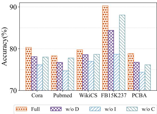
As shown in Figure 3, the “Full” model is the orange bar with the stars. In almost every case, removing a component drops performance. Removing the Invariant module (w/o I) causes a significant drop, highlighting that simply searching for architecture without separating invariant signals from noise leads to poor generalization.

Conclusion and Implications

AutoGFM represents a significant step forward in Graph AI. It addresses the inherent tension between the “Foundation Model” goal (one model for everything) and the “Graph Learning” reality (every graph is unique).

By leveraging a disentangled encoder to identify structural needs and a customizable super-network, AutoGFM allows a single model to fundamentally reshape itself—metaphorically changing its outfit—depending on whether it’s looking at a social network or a chemical compound.

For students and researchers, this paper highlights a critical lesson: Adaptability is key. As we build larger and more general models, the ability to dynamically adjust internal processing mechanisms based on the input context will likely become a standard requirement, moving us beyond the era of static neural architectures.