Mathematics is often viewed as a discipline of rigid logic and absolute proofs. A statement is either true or false; a theorem is proven or unproven. However, the process of reaching a proof is frequently messy, relying on intuition, visualization, and trial-and-error.

In recent years, a fascinating question has emerged: Can Artificial Intelligence act as an intuition engine for pure mathematics? Can it “dream up” geometric constructions that human mathematicians have overlooked?

A recent paper titled “Neural Discovery in Mathematics: Do Machines Dream of Colored Planes?” by Mundinger et al. answers this with a resounding “yes.” The researchers tackled the Hadwiger-Nelson problem, a notorious puzzle at the intersection of discrete geometry and combinatorics. By treating this rigid coloring problem as a fluid, continuous optimization task, they utilized neural networks to discover novel mathematical structures.

In this deep dive, we will explore how they reformulated a 70-year-old math problem into a loss function, the architectures they used to “paint” the plane, and the specific, novel colorings they discovered that improve upon decades of human effort.

The Problem: Coloring the Infinite

To understand the contribution of this paper, we first need to understand the Hadwiger-Nelson (HN) problem. First posed in 1950, the problem is deceptively simple to state:

What is the minimum number of colors needed to color the Euclidean plane (\(\mathbb{R}^2\)) such that no two points at a distance of exactly 1 unit share the same color?

This number is denoted as \(\chi(\mathbb{R}^2)\), the chromatic number of the plane.

Imagine holding a rigid stick of length 1. No matter where you place this stick on an infinite sheet of paper, the two ends must land on different colors.

Despite its simplicity, the problem remains unsolved.

• Lower Bound: We know we need at least 5 colors (a result established only recently in 2018 by Aubrey de Grey).
• Upper Bound: We know 7 colors are sufficient (proven in 1950 via a hexagonal tiling).

The answer is 5, 6, or 7. Narrowing this gap has proven incredibly difficult because the problem mixes discrete choices (assigning distinct colors) with continuous geometry (the infinite plane with uncountably many points) and hard constraints (the unit distance rule).

Traditional computational methods, like SAT solvers, struggle here because they require discretizing the plane into a grid, which loses the nuances of continuous geometry. This is where the authors’ “Neural Discovery” approach steps in.

The Core Method: Softening the Hard Constraints

The authors’ primary innovation is reformulating this rigid coloring problem into a continuous optimization task that a neural network can solve via gradient descent.

From Discrete to Probabilistic

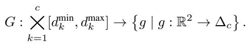
In a standard coloring, a point \(x\) is assigned a specific color \(c\). Mathematically, this is a function \(g: \mathbb{R}^2 \rightarrow \{1, \dots, c\}\) that satisfies the condition:

This discrete function is non-differentiable; you cannot easily compute a gradient to “nudge” a point’s color in the right direction. To fix this, the researchers relax the constraint. Instead of a hard color assignment, they assign a probability distribution over \(c\) colors to each point in the plane.

They define a mapping \(p: \mathbb{R}^2 \to \Delta_c\), where \(\Delta_c\) is the probability simplex for \(c\) colors. For example, if we are testing for 6 colors, the network outputs a vector of 6 probabilities for any given coordinate \((x, y)\).

If the dot product \(p(x)^T p(y)\) is high, it means points \(x\) and \(y\) have a high probability of being the same color. If the dot product is 0, they are definitely different colors.

The Geometric Loss Function

The heart of this method is the loss function. The goal is to minimize the probability that any two points separated by distance 1 share the same color. Since checking every pair of points in an infinite plane is impossible, they restrict the optimization to a large finite box \([-R, R]^2\).

The loss function \(\mathcal{L}_R(p)\) is defined as an integral:

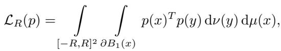
Let’s break down this equation, as it is the engine of the entire discovery process:

1. \(\int_{[-R, R]^2} ... d\mu(x)\): The outer integral iterates over every “center” point \(x\) in our bounding box.
2. \(\int_{\partial B_1(x)} ... d\nu(y)\): The inner integral looks at the “sphere” (circle) of radius 1 around \(x\). These are all the points \(y\) that are exactly 1 unit away from \(x\).
3. \(p(x)^T p(y)\): This measures the “collision.” It is the probability that \(x\) and \(y\) share a color. We want this to be zero.

The objective is simple: find the probabilistic coloring \(p\) that minimizes this loss.

Implicit Neural Representations

To solve this, the authors use a Neural Network as a function approximator. The network takes a 2D coordinate \((x, y)\) as input and outputs the color probability vector. This setup is known as an Implicit Neural Representation.

The architecture is a standard Multi-Layer Perceptron (MLP) with sine activation functions. Why sine waves? Unlike ReLUs, sine activations give the network a “spectral bias,” meaning it naturally favors learning smooth, periodic functions. Since many geometric colorings (like grids or honeycombs) are periodic, this architecture is perfectly suited for the task.

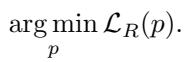
Training via Monte Carlo Sampling

Calculating the double integral in the loss function exactly is computationally intractable. Instead, the researchers approximate the gradient using Monte Carlo sampling.

In every training step:

1. They sample \(n\) random points (\(x_i\)) inside the box.
2. For each \(x_i\), they sample \(m\) random points (\(y_{ij}\)) on the unit circle around it.
3. They calculate the collision probability.
4. They backpropagate the error to update the network weights \(\theta\).

This allows the network to explore the space of colorings. Initially, the coloring is random noise. Over thousands of iterations, the network “dreams” of patterns—stripes, waves, and hexagons—that minimize unit-distance conflicts.

Case Study 1: Almost Coloring the Plane

One of the most interesting variations of the Hadwiger-Nelson problem asks: If we are only allowed \(k\) colors (where \(k < \chi(\mathbb{R}^2)\)), what is the smallest fraction of the plane we must leave uncolored to avoid conflicts?

This is the “Almost Coloring” problem. The goal is to color as much of the plane as possible with a limited palette.

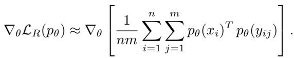
The Lagrangian Relaxation

To solve this, the authors introduce a “bonus” color (let’s call it the “trash” color). Points assigned to this trash color don’t trigger unit-distance conflicts, but using this color is penalized.

They formulate a constrained optimization problem:

Here, the \((c+1)\)-th color is the trash color. The constraint ensures the total area of the trash color stays below a threshold \(\delta\). In practice, they convert this into a Lagrangian relaxation:

The parameter \(\lambda\) controls the trade-off. If \(\lambda\) is high, the network fights hard to minimize the uncolored area.

From Neural Dreams to Formal Proofs

One of the key themes of this paper is that the neural network’s output is not a proof; it is a candidate. The network might output a coloring that looks perfect to the naked eye but has microscopic errors (0.01% conflicts).

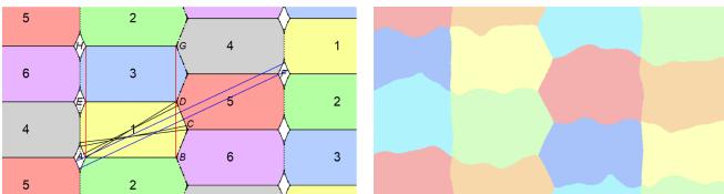
To turn these “dreams” into math, the authors developed an automated pipeline (Algorithm 1) to formalize the results.

1. Initial Training: Train the network to find a low-conflict pattern.
2. Periodicity Extraction: Analyze the image to find the repeating “tile” (a parallelogram).
3. Retraining: Train a new network that is forced to be periodic on that specific tile.
4. Discretization: Convert the continuous probability map into a discrete grid of pixels.
5. Conflict Resolution: Use a discrete algorithm (minimum edge cover) to clean up the remaining pixels that cause conflicts, assigning them to the “trash” color.

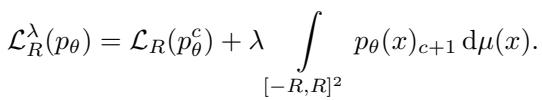
The results were impressive. For the 5-color variant, previous best constructions left about 4.01% of the plane uncolored. The neural network found a pattern that only required removing 3.74% of the plane.

Figure 10 below shows the evolution of these patterns as the algorithm iterates, clarifying the fundamental parallelogram domain (the box) that tiles the plane.

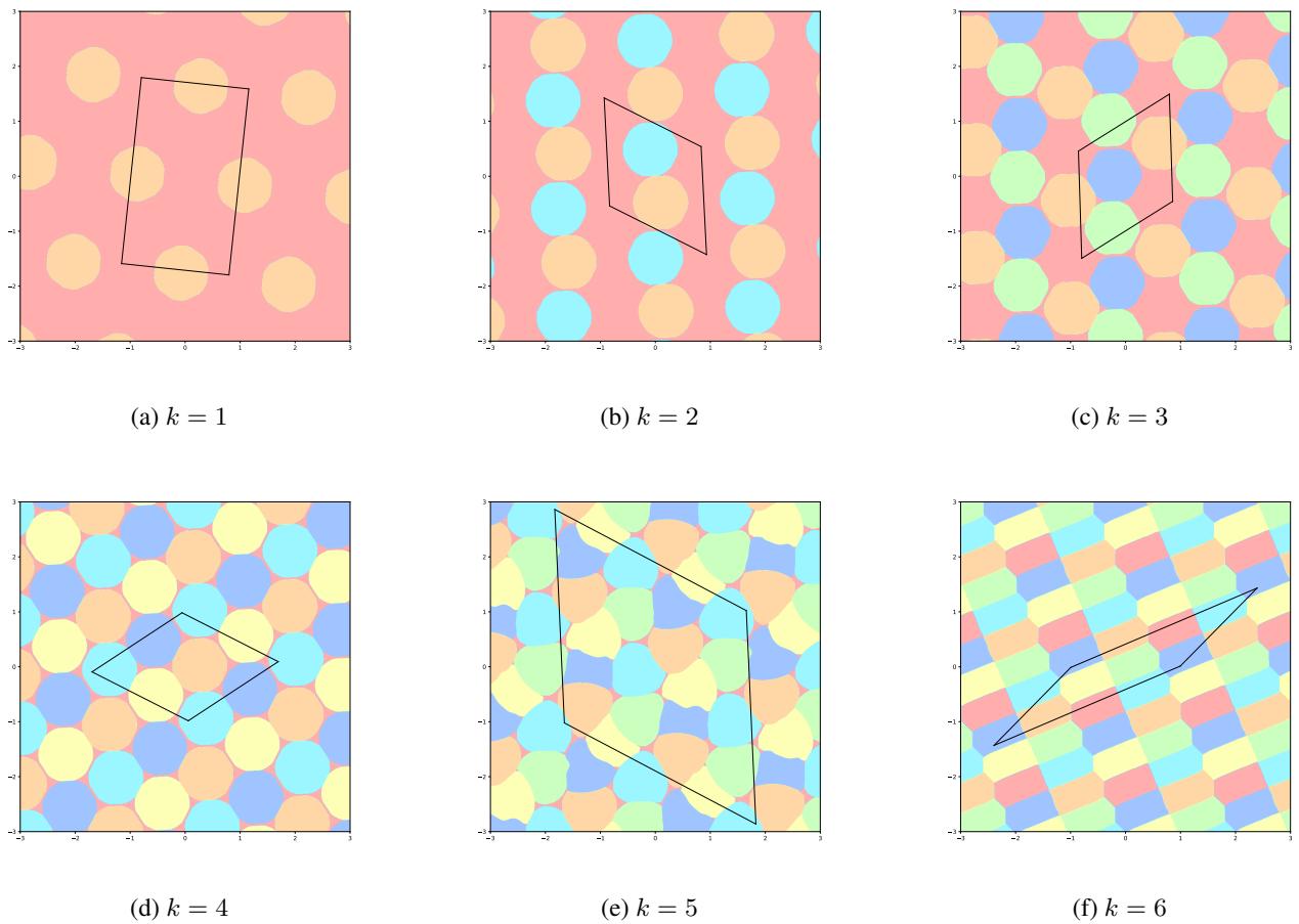
The final formalized result for 5 colors is a complex, beautiful structure. Figure 2 shows this “almost 5-coloring.” The red areas represent the uncolored “trash” regions.

Notice the “wavy” boundaries in the left comparison below (Figure 5). The network often produces organic, fluid shapes because there are degrees of freedom in the solution space.

Case Study 2: The Off-Diagonal Discovery

The most significant theoretical contribution of the paper involves a variant called the “Off-Diagonal” Hadwiger-Nelson problem.

In the standard problem, every color must avoid distance 1. In the off-diagonal version, different colors avoid different distances. A coloring of type \((d_1, d_2, \dots, d_k)\) means color 1 avoids distance \(d_1\), color 2 avoids distance \(d_2\), and so on.

The researchers searched for a 6-coloring of type \((1, 1, 1, 1, 1, d)\). This means 5 colors avoid unit distances, and the 6th color avoids some distance \(d\).

Extending the Continuum

For over 30 years, the range of valid distances \(d\) for which such a coloring existed was stuck in a specific interval. The researchers trained their networks to sweep across different values of \(d\), looking for regions where the loss function dropped to zero.

To do this efficiently, they fed the distance \(d\) as an input to the neural network along with the coordinates. This allowed a single network to learn the solution for the entire continuum of distances at once.

The results were a breakthrough. They found two new distinct 6-colorings.

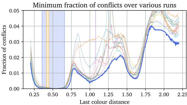
The First Coloring (Variable \(d\)): They discovered a family of colorings valid for \(0.354 \leq d \leq 0.553\). The graph below (Figure 6) plots the conflict rate against the distance \(d\). The blue shaded region represents the new range of solutions discovered by the AI, significantly extending the previously known orange region.

The Second Coloring (Fixed Range): They also found a specific pattern that works for any \(d\) between 0.418 and 0.657.

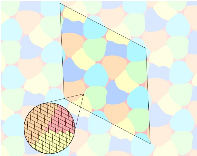
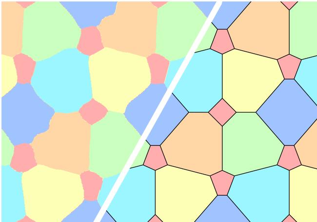
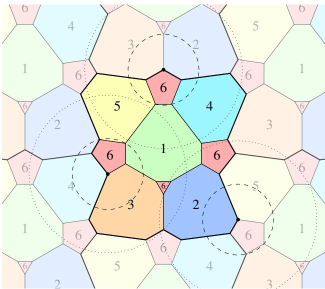
This is where the “visual discovery” aspect shines. Figure 1 shows the raw output of the neural network on the left. It looks like a noisy, pastel stained-glass window. On the right is the human-formalized construction derived from interpreting that noise.

The formalized version (Figure 11 below) reveals a clever tessellation of polygons. The red color (color 6) is carefully placed to avoid the specific distance range, while the other colors handle the unit distances.

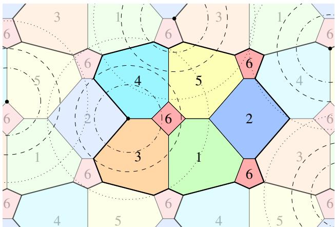
Figure 3 visualizes the constraints for a specific instance (\(d=0.45\)). The red points are spaced such that they never fall on the dashed circle (radius 0.45).

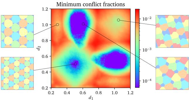
They also explored colorings where two colors have non-unit distances \((1, 1, 1, 1, d_1, d_2)\). By plotting the conflict minima on a heatmap (Figure 7), they identified islands of stability—regions where valid colorings are likely to exist. This acts as a treasure map for mathematicians, pointing them exactly where to look for proofs.

Case Study 3: Avoiding Monochromatic Triangles

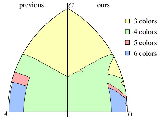
The HN problem deals with pairs of points. A harder variant asks: How many colors are needed to avoid monochromatic triangles of specific side lengths?

Specifically, can we color the plane such that no three points forming a triangle with side lengths \((1, a, b)\) are all the same color?

To tackle this, the authors modified the loss function to look at triplets of points.

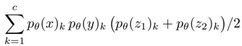
Here, \(z_1\) and \(z_2\) are the points that form the specific triangle with points \(x\) and \(y\).

The results provided a massive update to the known bounds. In Figure 4 below, the left chart shows the “Previous” state of knowledge. The colored regions represent triangle dimensions \((a, b)\) solvable with 3, 4, 5, or 6 colors. The right chart shows the “Ours” result.

Notice how the regions for 3 and 4 colors (yellow and green) have expanded significantly. The AI found stripe-based patterns and hexagonal tessellations that humans hadn’t optimized for these specific triangle shapes.

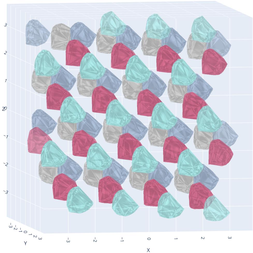
Exploring Higher Dimensions

Finally, the authors took their framework into 3D space (\(\mathbb{R}^3\)). The “Chromtic Number of Space” is known to be at most 15. The authors’ method successfully found conflict-free 15-colorings.

Visualizing 3D colorings is difficult, but the neural network handles the extra dimension effortlessly—it’s just another input node. Figure 15 shows a slice of a discovered 3D coloring, revealing gemstone-like polyhedral structures.

Conclusion: The Future of AI in Mathematics

The paper “Neural Discovery in Mathematics” is a compelling demonstration of the AI-for-Science paradigm. It does not replace mathematicians; rather, it augments them.

The workflow established here is powerful:

1. Reformulate a discrete problem into a differentiable loss function.
2. Train a neural network to find approximate solutions (the “dreaming” phase).
3. Interpret the visual patterns to derive formal mathematical constructions.
4. Verify the constructions using rigorous logic.

The authors used this to improve bounds on the Hadwiger-Nelson problem that had stood for decades. The neural networks didn’t just crunch numbers; they acted as microscopes, revealing geometric structures in the continuum that were previously invisible to human intuition. As these techniques refine, we may find that machines don’t just dream of colored planes—they might dream up the theorems of the future.